Matlab辨识工具箱里面的函数很多,这里用一个简单的例子来展示估算系统传递传递函数的使用方法。
比如我们的任务是,已知系统的输入输出,而系统未知,是个黑盒子,需要我们去估算系统的传递特性。
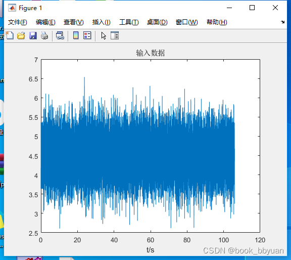
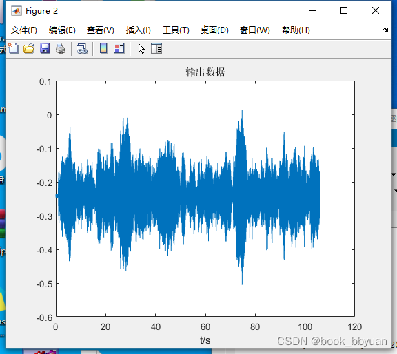
我们的系统输入输出数据如下
系统未知,我们通过 功率谱估算 来求解系统响应
Transfer function estimate - MATLAB tfestimate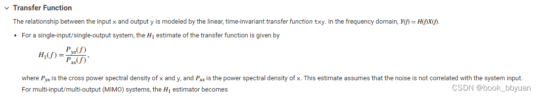
互功率谱和自功率谱相除就得到了系统频响
[pxx,f1] = pwelch(x,window,noverlpap,Nfft,fs);
[pyx ,f2]= cpsd(y,x,window,noverlpap,Nfft,fs);
tfunc=pyx./pxx;
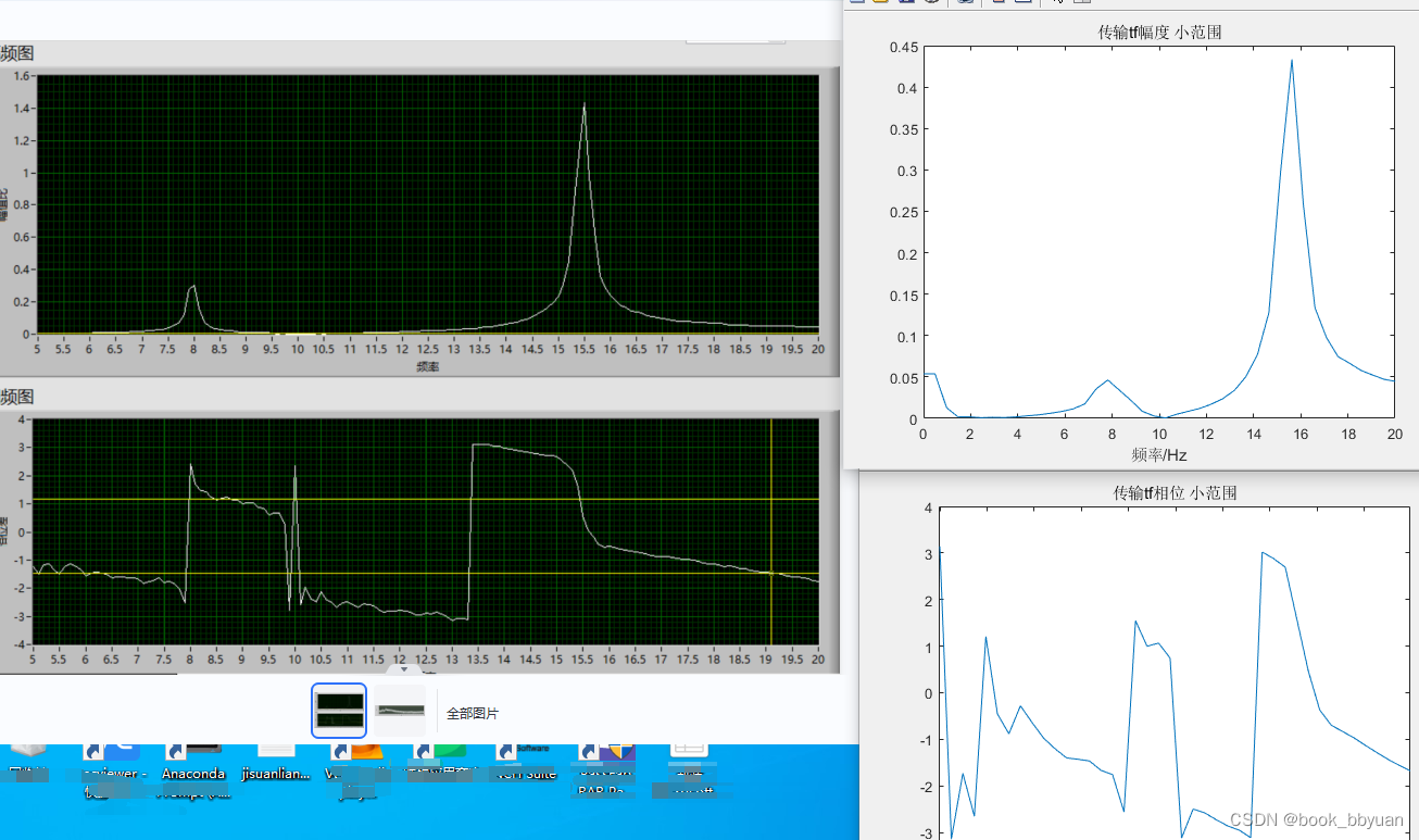
我们得到系统频响(幅度和相位)
plot(f,(abs(tfunc)));
title('传输tf幅度 小范围');
xlim([0,20]);
plot(f,(angle(tfunc)));
title('传输tf相位 小范围');
xlim([0,20]);
ypf = angle(tfunc);
这刚好和我们用 得到的 频响是一致的
下面估算系统的传递函数
Create Frequency Response Object
sysfr = idfrd(ResponseData,Frequency,Ts)idfrd object that stores the frequency response ResponseData of a linear system at frequency values Frequency. Ts is the sample time. For a continuous-time system, set Ts to 0.
sys = arx(data,[na nb nk]) estimates the parameters of an ARX or an AR idpoly model sys using a least-squares method and the polynomial orders specified in [na nb nk]. The model properties include covariances (parameter uncertainties) and goodness of fit between the estimated and measured data.
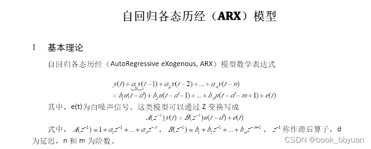
上na nb nk分别是,分母系数个数,分子系数个数和delay
很遗憾,我们也不具体了解这个未知系统的 零极点个数(或者说多项式的阶数)
ypf = abs(tfunc);
xpf = f;
frdobj = idfrd(ypf,xpf,1/fs);
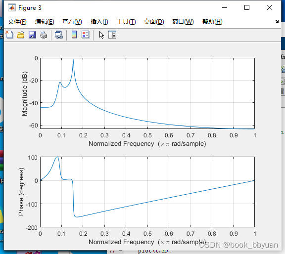
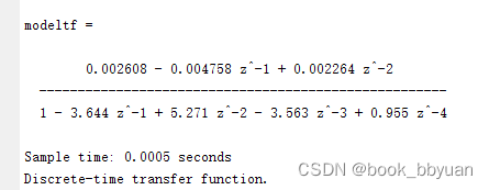
modelobj = arx(frdobj,[4 3 0])
modeltf = tf(modelobj);
b = cell2mat(get(modeltf,'Numerator'));
a = cell2mat(get(modeltf,'Denominator'));
估算的系统响应,已经把两个峰值的特性 仿真出来了
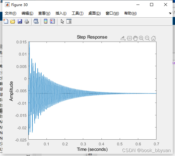
单位冲击
step(modeltf)
传递函数
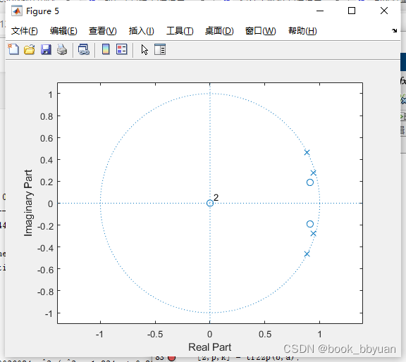
零极点形式
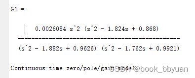
zplane 零极点图