《合成孔径雷达成像——算法与实现》之【6】仿真图3.6加窗

版权声明：本文为博主原创文章，未经博主允许不得转载。 https://blog.csdn.net/Destiny0321/article/details/53219053

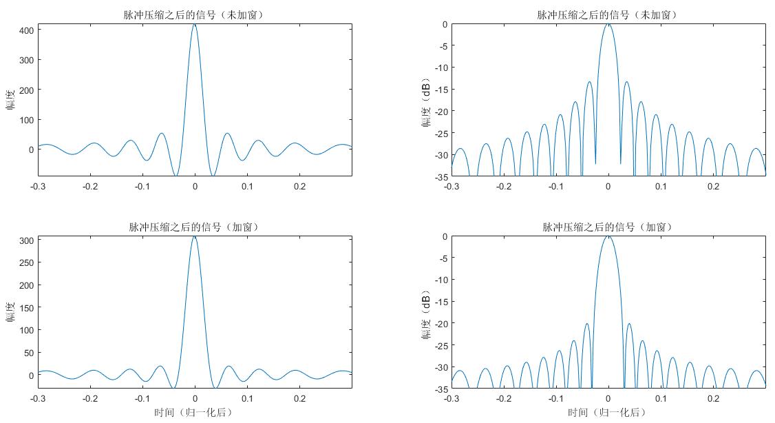
这里主要对图3.6的匹配滤波器作了加窗（Kaiser窗）处理，使得脉冲压缩效果有了变化：加窗之后的信号幅度较未加窗信号有了降低，但峰值旁瓣比下降了7dB。

% SAR_Figure_3_6_window
% 匹配滤波器加窗和不加窗的效果对比
% 2016.08.31

close all;clear all;clc

T = 7.24e-6;                                        % 信号持续时间
B = 5.8e6;                                          % 信号带宽
K = B/T;                                            % 调频率
ratio = 10;                                         % 过采样率
Fs = ratio*B;                                       % 采样频率
dt = 1/Fs;                                          % 采样间隔
N = ceil(T/dt);                                     % 采样点数
t = ((0:N-1)-N/2)/N*T;                              % 时间轴

st = exp(1i*pi*K*t.^2);                             % 生成信号
ht = conj(fliplr(st));
window = kaiser(N,2.5)';
ht_window = window.*conj(fliplr(st));               % 匹配滤波器

Sf = fftshift(fft(fftshift(st)));
Hf = fftshift(fft(fftshift(ht)));
Hf_window = fftshift(fft(fftshift(ht_window)));

out = ifftshift(ifft(ifftshift(Sf.*Hf)));
out_window = ifftshift(ifft(ifftshift(Sf.*Hf_window)));

Z1 = abs(out);
Z1 = Z1/max(Z1);
Z1 = 20*log10(Z1);

Z2 = abs(out_window);
Z2 = Z2/max(Z2);
Z2 = 20*log10(Z2);

tt = linspace(-0.5,0.5,N);
figure,set(gcf,'Color','w');
subplot(2,2,1),plot(tt,out);axis([-0.3 0.3 -inf inf]);
title('脉冲压缩之后的信号（未加窗）'),ylabel('幅度');
subplot(2,2,2),plot(tt,Z1);axis([-0.3 0.3 -35 inf]);
title('脉冲压缩之后的信号（未加窗）'),ylabel('幅度（dB）');
subplot(2,2,3),plot(tt,out_window);axis([-0.3 0.3 -inf inf]);
title('脉冲压缩之后的信号（加窗）'),xlabel('时间（归一化后）'),ylabel('幅度');
subplot(2,2,4),plot(tt,Z2);axis([-0.3 0.3 -35 inf]);
title('脉冲压缩之后的信号（加窗）'),xlabel('时间（归一化后）'),ylabel('幅度（dB）');