《合成孔径雷达成像——算法与实现》之【3】仿真图3.2

版权声明：本文为博主原创文章，未经博主允许不得转载。 https://blog.csdn.net/Destiny0321/article/details/53096089

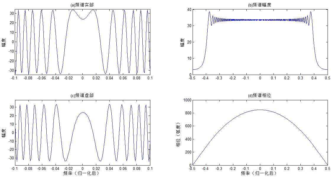
为了对线性调频信号的频域性质有更清晰的认识，将信号持续时间T = 7.24us保持不变，而将信号带宽提升到B = 99.43MHz，过采样率降至1.25。可以看到，在频域中信号的实部和虚部也具有线性调频结构。

% SAR_Figure_3_2
% 2016.10.12

close all;clear all;clc

T = 7.24e-6;                % 信号持续时间
B = 99.43e6;                % 信号带宽
K = B/T;                    % 调频率
ratio = 1.25;               % 过采样率
Fs = ratio*B;               % 采样频率
dt = 1/Fs;                  % 采样间隔
N = ceil(T/dt);             % 采样点数
t = ((0:N-1)-N/2)/N*T;      % 时间轴

st = exp(1i*pi*K*t.^2);     % 生成信号
Sf = fftshift(fft(fftshift(st))); % FFT

tt = linspace(-0.5,0.5,N);
figure,set(gcf,'Color','w');
subplot(2,2,1),plot(tt,real(Sf));axis([-0.1 0.1 -inf inf]);
title('(a)频谱实部'),ylabel('幅度');
subplot(2,2,2),plot(tt,abs(Sf));
title('(b)频谱幅度'),ylabel('幅度');
subplot(2,2,3),plot(tt,imag(Sf));axis([-0.1 0.1 -inf inf]);
title('(c)频谱虚部'),xlabel('频率（归一化后）'),ylabel('幅度');
subplot(2,2,4),plot(tt,unwrap(angle(Sf)));
title('(d)频谱相位'),xlabel('频率（归一化后）'),ylabel('相位（弧度）');