Coursera: Algorithms part 1 Week 1

Union-Find

dynamic connectivity
quick find
quick union
improvments to make the tree flat

weighted quick-union
path-compression

application: percolation

Analysis of Algorithms

introduction
observations
mathematical models
order-of-growth algorithms

二分法查找
An $N^2\log N$ algorithms for 3-Sum

theory of algorithms

三种记号

memory

Union-Find

这节课从应用的角度出发，讲解广泛应用的union-find（UF）。

dynamic connectivity

Model
功能：实现N个对象的连接操作
判断两个对象是否连接。
比如，0-9 以整数序号代表10个对象。
Application
路径是否连通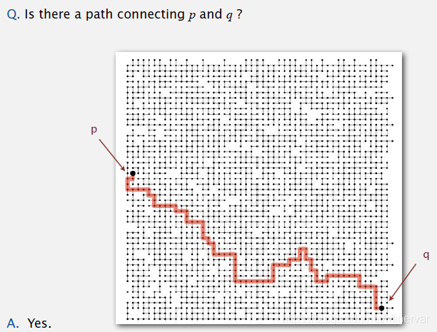
其他类型的应用包括：
照片的像素点位
网络中的计算机
社会网中的人际关系
电脑芯片中的晶体管
数学集合中的元素（abstract: When we process a pair p q, we are asking whether they belong to the same set. If not, we unite p’s set and q’s set, putting them in the same set.）
Fortran程序中的变量（是否引用了同一个对象）等
API and client

// API pseudocode 
public class UF
{
UF(int N)			 //初始化
void union(int p, int q)	//union 
boolean connected(int p, int q) 	//connected
int find(int p)
int cout()
}

//Client real code
public static void main(String[] args)
{
	int N = StdIn.readInt();
	UF uf = new UF(N);
	while (!StdIn.isEmpty())
	{
		int p = StdIn.readInt();
		int q = StdIn.readint();
		if (!uf.connected(p,q))
		{
			uf.union(p,q)
			StdOut.println( p + " " + q);
		}
	}
}

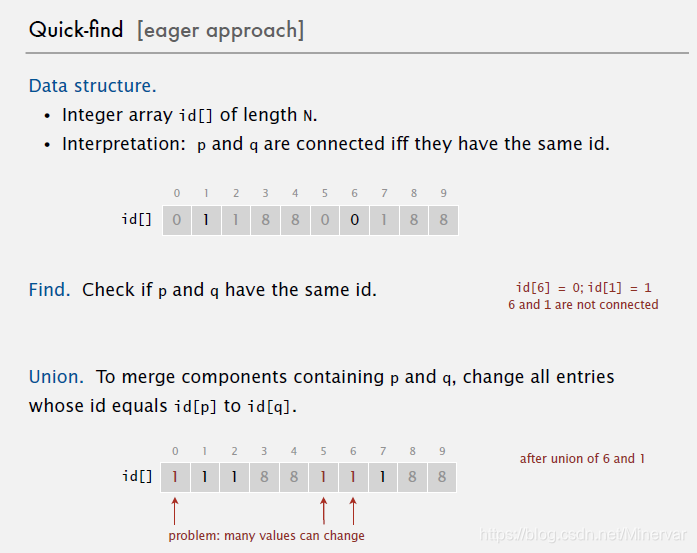
quick find

使用java内置的数列，id[index] = value。这里不同的index表示不同的对象，对应value表示所属的集合数。
connected(p, q) 即，slide中的Find，这个方法的实现比较简单：直接检查id[p]是不是等于id[q]
union(p, q) 这个方法比较复杂：在连接两个集合时候，需要对整个序列进行遍历，找到并改变属于其中一个集合的对象的value。
在这里插入图片描述
实现的代码如下：

public class QuickFindUF
{
	private int[] id;
	public QuickFindUF(int N)
	{
		id = new int[N];
		for (int i = 0; i < N; i++)
		{
			id[i] = i;  // 必须进行初始化，指向自己
		}
	}
	public boolean connected(int p, int q)
	{
		int pid = id[p];
		int qid = id[q];
		for (int i = 0; i < id.length; i++) // 遍历一遍数组 找到 p 同属一个集合的所有元素 都合并到 q 所在的集合中
		{
			if (id[i]==pid) id[i] = qid;
		}
	}
}

算法分析
在这里插入图片描述
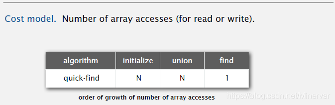
quick-find在union操作上面时间开销太大了。
如果对N个对象进行N次Union操作，那么时间成本是 $N^2$ (quadratic time)。
为什么quadratic time不行呢？

实际例子
现代计算机大概每秒运行 $10^9$ 次，可存储 $10^9$ 个单词在主存中。如果对这些对象进行操作 $10^9$ 次union，Quick-find 需要 $10^18$ ，30多年的时间。
Quadratic algorithms don’t scale with technology.
现代计算机的计算速度增加了10倍，但是与此同时内存也增加了10倍；同时，我们想解决的问题也是10倍的复杂度。但是quadratic algorithms的时间开销也需要10倍那么长。我的理解是 $\frac{10M \times 10N} {10} = 10 MN$ 。这种算法只有当N的上限比较小时或者不需要频繁执行才是可行的。

quick union

这里构造了一个树状的结构。对比quick find的算法，id[index] = value，这里的value表示的不是同一个节点而是上一级对象的节点。
在这里插入图片描述
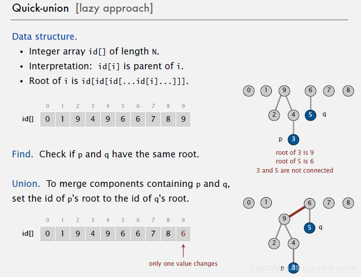
那么在操作上，
connected (Find): 只需要比较最终的根节点是否一样。这里会多出一个root的方法找每个对象的根节点。
union: 则是把两个节点的根节点直接连接起来。

public class QuickUnionUF
{
	private int[] id;  \\ 内部变量声明
	public QuickUnionUF(int N)
	// 对象QuickUnionUF初始化
	{
		id = new int[N];
		for (int i = 0; i < N; i++) id[i] = i;
		// 将每个变量的id[index] 初始化设为自身序号index
	}
	private int root (int i)
	// root 函数
	// 输入变量 为节点序号
	// 输出变量 为根节点序号
	{
		while (i != id[i]) i = id[i];
		return i;
	}
	public boolean connected (int p, int q)
	\\ 判断两个节点是否相等
	{
		return root(p) == root(q);
	}
	public void union  (int p, int q)
	\\ 将p的根节点与q根节点连接起来
	\\连接方式为将p的根节点的上一级节点指向q
	{
		int i = root(p);
		int j = root(q);
		id[i] = j;
	}
}

算法分析

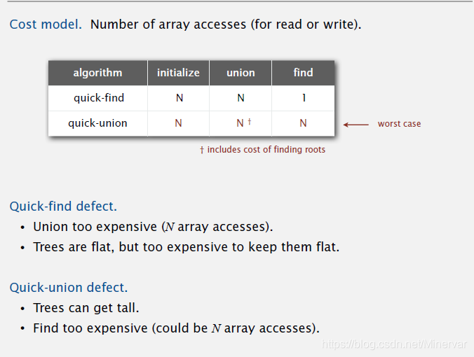
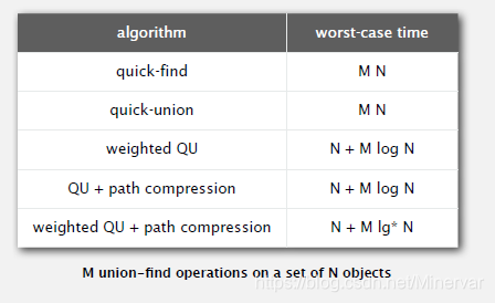
对比上来看，在最差的情形下（平均情况，quick-union的union操作是要比quick-find小的。），quick-union的时间开销也很大。从操作上来看，主要是找到根节点需要的时间比较大；查询时间与所生成的树的形状有很大关系。树如果越扁平，查询根节点的时间越小。

improvments to make the tree flat

针对上一节提出的树的形状问题，这一节lecture里面提到了两个可以让树变得扁平的方法。

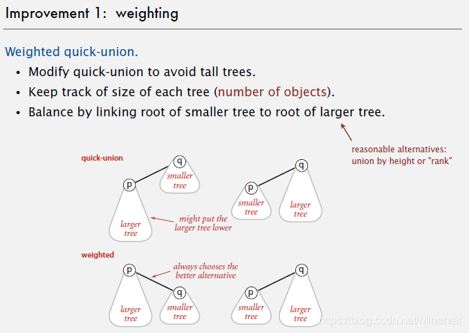
weighted quick-union

思路：在连接两个根节点的时候，只选择把小数的根节点连接在大树上。
那么，这就需要我们在类中加入数组记录每一个节点所在的树的大小。

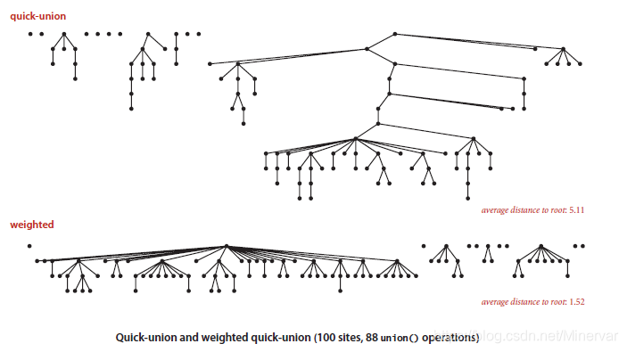
模拟的实验结果表明，weighting的方法生成的树平均深度要比单纯的quick-union小。
comparison
程序上，只需要增加private int[] sz并且修改方法union中连接根节点的代码段：

public void union (int p, int q)
{
	int i = root(p);
	int j = root(q);
	if (i==j) return;
	if (sz[i] < sz[j])	{id[i] = j; sz[j] += sz[i];}
	else				{id[j] = i; sz[i] += sz[j];}
}

在运行时间上
Find，所需时间是与节点的深度成正比例
Union，再给定root的情况下，需要常数时间
root，root的时间也与节点的深度成正比例
weighting的方法：给出的树的最大深度不超过 $\log_2 N$ 。（可用反证法证明）

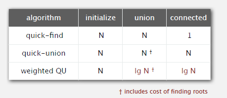
三种算法的时间开销比较：
comparison

path-compression

在运行root方法的时候，将所查询元素的上一级节点直接设置为根节点。
通过简单地改变root函数：
让每一个路径节点指向自己的祖父节点。

private int root(int i)
{
	while (i ! = id[i])
	{
		id[i] = id[id[i]];
		i = id[i];
	}
	return i;
}

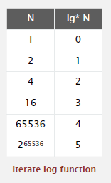
四种算法的时间开销比较：
在这里插入图片描述
需要解释一下的是 $\log\star$ 函数。
logStar

application: percolation

percolation是一个比较常见的物理系统。

存在一个临界的概率 $~p^{\star}$ ，使得percolated的概率突然增加。
percolationProbability
对于这个没有数值解的情况，往往需要蒙特卡洛进行模拟。（这是本周的编程作业。）
Lecture中，老师给出了利用UF写作业的思路：
把两端的open site看成连接到某个虚拟的根节点上，那么判断是否percolate相当于判断这两个虚拟节点是否是连通的。
clever trick

Analysis of Algorithms

introduction

Reasons to analyze algorithms
predict performance
compare algorithms
provide guarantees --the worst case
understand theoretical basis
Cases
2.1 Problem: Fourier transformation
Desription: Break down waveform of N samples into periodic components.
Applications: DVD,JPEG, MRI ect.
Brute force: $N^2$ steps
FFT algorithmn: $N\log N$ steps, enables new technology.
2.2 Problem: N-body simulation
Description: Simulate gravitational interactions among N steps
Brute force: $N^2$ steps
Barnes-Hut algorithms: $N\log N$ steps, enables new research.
Framework to understand performance
这也是一般科学研究的步骤
3.1 Observe some feature of the natural world
3.2 Hypothesize a model that is consistent with the observations
3.3 Predict events using hypothesis.
3.4 Verify the predictions by making further observations
3.5 Validate by repeating until the hypothesis and observation agree

observations

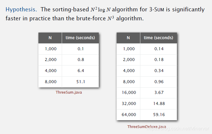
本节用3-Sum这个问题的最一般解法作为例子来解释程序运行的时间开销问题。
Example：3-sum
问题描述：给定不同的N个整数，其中有多少个三元组的和为0（三元组的所有元素均来自于N个整数且为不同元素）。
Brute force：暴力解法

public class ThreeSum
{
	public static int count(int[] a)
	{
		int N = a.length;
		int count = 0;
		for (int i = 0;i <N; i++)
		{
			for (int j = i+1; j <N; j++)
			{
				for (int k = j+1; k < N; k++)
				{
					if (a[i]+a[j]+a[k] == 0)
					count++l
				}
			}
		}
	}
	return count;
}
public static void main(String[] args)
{
	int[] a = In.readInts(args[0]);
	StdOut.println(count(a)); // 这里不需要生成ThreeSum的对象就直接调用吗？
}

在给定N的情况下，如何给这个程序计时呢？
手动计算时间：
ticktock
内置Stopwatch类计算时间：

public static void main(String[] args)
{
	int[] a = In.readInts(args[0]);
	Stopwatch stopwatch = new Stopwatch();  // 时间计算的起点
	StdOut.println(ThreeSum.count(a));
	double time = stopwatch.elapsedTime(); // 时间计算终止，中间过程时间间隔存放在变量time中
}

** Observation–Data Analysis**
如何对时间开销进行分析？
经过多次计算（N，T(N)），可以画出运行时间 T(N)和数据大小N的图像。
standard plot
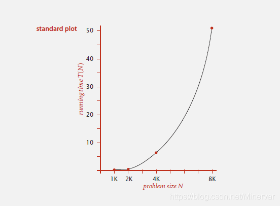
疑似指数关系，重新作出log-log图像。
log-log
进行图形拟合之后， $b\approx 3$ 与推测相吻合。
Hypothesize
我们也得到了可以用来估计运行时间的方程：
$T(N)\approx 1.006\times 10^{-10}\times N^{2.999}$ 。
Predictions and further observation

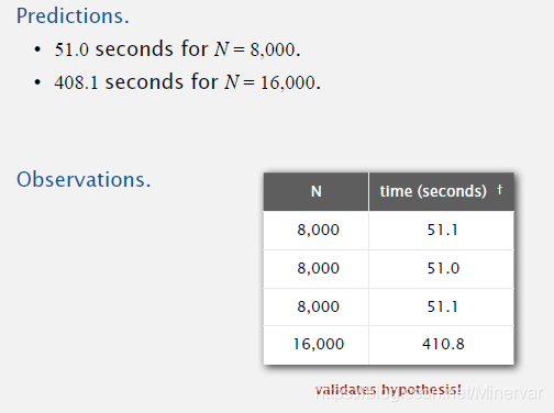
Alternative hypothesis: Doubling hypothesis 一个快速估计 $b$ 的方法：

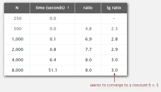
可以看到用于实验的 $N$ ，是倍数关系。第三列计算的是当前 $\frac{T(2N)}{T(N)}$ 。取这个值的对数（表格中是以2为底数），可以直接得到 $b$ 的值。
缺陷这种方法并不能直接得出 $a$ 的值。 $a$ 的值可以间接计算得出。这种方法得到的方程为：
$T(N) \approx 0.998\times 10^{-10}\times N^3$ 。
附注：这些运算的结果会因为计算机的不同有差异，这里所用的时间单位是秒。
影响运行时间的因素

系统无关变量：算法与输入数据
系统相关变量：CPU、软件、系统

comments：
虽然不能达到精确的测量，但计算实验比分析方法更简单易行。

mathematical models

这一节老师讲解了数学上的理论分析方法:
首先，Principle:

$total running time = \sum_{all operartions} cost \times frequency $;
精确运行时间的测量是可行的。

举了两个例子来说明如何计算：

case1： 1-sum

int count = 0;
for (int i = 0; i<N; i++)
{
	if(a[i] == 0) count ++;
}

在这个例子中，
在这里插入图片描述

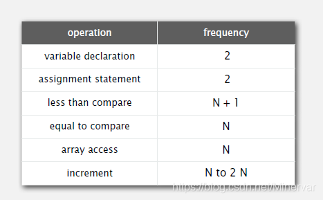
case2：2-sum

int count = 0;
for (int i=0; i< N; i++)
{
	for (int j=0; j<N;j++)
	if (a[i] + a[j] ==0)
		count++;
}

在这个例子中，
在这里插入图片描述
这种计算过程过于复杂。
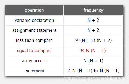
Simplification

只分析最大的
在2-sum这个例子中，只分析“equal to compare”这个操作。
tilde notation （等价无穷大）
Ex1: $\frac{1}{6}N^3 + 20N + 16 \sim \frac{1}{6} N^3$
Ex2: $\frac{1}{6}N^3 + 100N^{4/3} + 56 \sim \frac{1}{6} N^3$
Ex3: $\frac{1}{6}N^3 -\frac{1}{2}N^{2} + \frac{1}{2}N \sim \frac{1}{6} N^3$
丢掉低阶项
所以，在2-sum这个例子中，

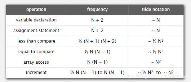
综合前面两种简化方式，得到2-sum的时间为 $\sim N^2$ 。
同样的方法，可以知道3-sum的时间为 $\sim \frac{1}{2} N^3$ 。

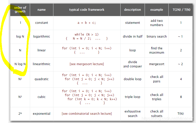
order-of-growth algorithms

这一节讲解运行时间函数的分类：
$1$ ， $\log N$ ， $N$ ， $N\log N$ ， $N^2$ ， $N^3$ ， $2^N$
在这里插入图片描述
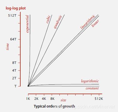
在摩尔定律下，线性或者是线性对数的算法复杂度才是可行的。

二分法查找

代码如下：

public static int binarySearch(int[] a, int key)
{
	int lo = 0; hi = a.length - 1;
	while (lo <= hi)
	{
		int mid = lo + (hi-lo)/2;
		if 	(key < a[mid]) hi = mid - 1;
		else if (key > a[mid]) lo = mid + 1;
		else return mid;
	}
	return -1;
}

这种算法的时间复杂度：
$T(N) \le T(N/2) + 1 \le T(N/4) +1 + 1 \le \dots \le T(N/N) + 1 +1 + \dots + 1 = 1 + \log N$

An $N^2\log N$ algorithms for 3-Sum

在了解了二分查找方法之后，我们可以进一步得到时间复杂度为 $N^2\log N$ 的算法解决3-sum问题。
Sorted-based algorithms

step 1: 将N个对象排序
step 2: 对于每一对数据 $(a[i],a[j])$ ，用二分法在完成排序之后的数组中查找 $-(a[i] + a[j])$ 。
分别对Step1和Step2进行分析，step1使用插入排序算法，时间复杂度为 $N^2$ ；step2的时间复杂度为 $N^2\log N$ 。
在分析的基础上可以得到假设：
排序基础上的3-sum算法比原来的暴力算法要快得多。
实验结果佐证了我们的假设：

theory of algorithms

回顾我们之前提到的，时间复杂度有两个与系统无关的影响因素：算法和数据。
对于同一种算法，输入的数据不同可能导致很不一样的运行结果。所以，在算法分析中，我们一般会讨论三种情形：
在这里插入图片描述
这节介绍算法分析的另外一个维度：最好，最坏和平均情况。
最好的情况下–lower bound on cost
最差的情况下–upper bound on cost
平均情况下–“Expected” cost
在实践中，往往会考虑最差的情况和在随机出现的一般情况（因为可以在对输入数据进行随机处理）。

三种记号

$\Theta$ ：同阶来区别算法。
$\Omega$ : 同阶或者高阶表示算法下界。
$\mathcal{O}$ : 同阶或者低阶表示算法上界。
举了几个例子来说明上界和下界怎么标记，不展开了。最后这一节说，本书的重点是在tilde-notation。因此不常见上面的三种记号。

memory

除了时间开销之外，内存上的开销也是我们应当给予考虑的。但是，现代计算机的内存已经不构成性能的限制条件了。老师给出了java中不同类型对应的不同存储空间：
在这里插入图片描述
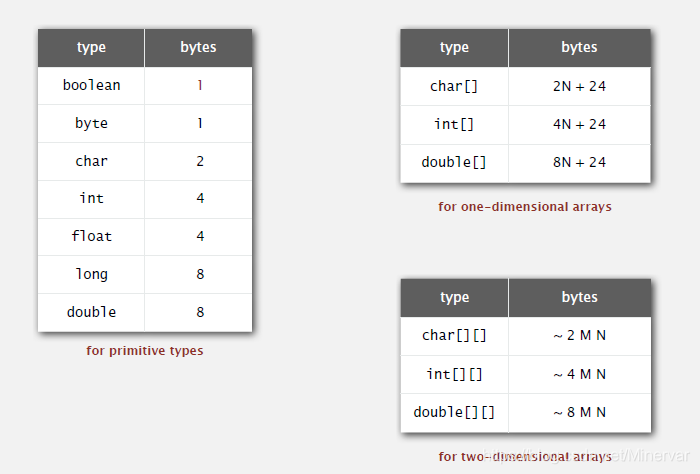
基本类型的空间开销需要记忆。
其中，
对象类型的固定空间开销为16 bytes。
对象引用的开销为8 bytes
padding 的开销为 8 bytes的倍数，（可能是0.5倍）。
举了很多计算的例子来说明这个的计算。
Ex.1

public class Date
{
	private int day; // 4 bytes
	private int month;// 4 bytes
	private int year; // 4 bytes
}

$16 ~bytes ~overhead + 3\times 4 ~bytes (int) + 4~ bytes (padding) = 32 ~bytes$

其他的计算不列举了。

Coursera: Algorithms part 1 Week 1

Coursera: Algorithms part 1 Week 1

Union-Find

dynamic connectivity

quick find

quick union

improvments to make the tree flat

weighted quick-union

path-compression

application: percolation

Analysis of Algorithms

introduction

observations

mathematical models

order-of-growth algorithms

二分法查找

An N 2 log ⁡ N N^2\log N N2logN algorithms for 3-Sum

theory of algorithms

三种记号

memory

猜你喜欢

An $N^2\log N$ algorithms for 3-Sum