PyImgSearch 博客中文翻译（二）

原文：PyImgSearch Blog

协议：CC BY-NC-SA 4.0

使用 TensorFlow 和 Keras 深入了解变形金刚:第 1 部分

原文：https://pyimagesearch.com/2022/09/05/a-deep-dive-into-transformers-with-tensorflow-and-keras-part-1/

---

目录

---

用 TensorFlow 和 Keras 深入了解变形金刚:第 1 部分

当我们看着人工智能生成的华丽的未来景观或使用大规模模型写我们自己的推文时，记住这一切从哪里开始是很重要的。

数据，矩阵乘法，用非线性开关重复和缩放。也许这简化了很多事情，但即使在今天，大多数架构都可以归结为这些原则。即使是最复杂的系统、想法和论文也可以归结为:

数据，矩阵乘法，用非线性开关重复和缩放。

在过去的几个月里，我们已经通过教程介绍了自然语言处理(NLP) 。我们从 NLP 的历史和基础出发，用注意力讨论神经机器翻译。

以下是按时间顺序排列的所有教程。

• 自然语言处理入门
• 介绍词袋(BoW)模型
• Word2Vec:嵌入 NLP 的研究
• BagofWords 和 Word2Vec 的比较
• 带 Keras 和 TensorFlow 的递归神经网络简介
• 长短期记忆网络
• 神经机器翻译
• 神经机器翻译用 Bahdanau 的注意力使用 TensorFlow 和 Keras
• 神经机器翻译用 Luong 的注意力使用 TensorFlow 和 Keras

现在，正如所讨论的，NLP 的进展讲述了一个故事。我们从记号开始，然后构建这些记号的表示**。我们使用这些表示来寻找记号之间的相似之处，并将它们嵌入到高维空间中。同样的嵌入也被传递到能够处理顺序数据的顺序模型中。这些模型用于构建上下文，并通过一种巧妙的方式，关注输入句子中对翻译中的输出句子有用的部分。

唷！做了很多研究。我们自己也差不多是一名科学家。

但是前方是什么呢？一群真正的科学家聚集在一起回答这个问题，并制定了一个天才计划(如图图 1 所示)，这将从根本上动摇深度学习领域。

在本教程中，你将了解导致变形金刚开创性架构的注意力机制的演变。

本课是关于 NLP 104 的三部分系列的第一部分:

1. 用 TensorFlow 和 Keras 深度潜入变形金刚:第一部 (今日教程)
2. 用 TensorFlow 和 Keras 深入了解变形金刚:第二部分
3. 使用 TensorFlow 和 Keras 深入了解变形金刚:第 3 部分

要了解注意力机制是如何进化成变压器架构的， 就继续阅读吧。

---

用 TensorFlow 和 Keras 深入了解变形金刚:第 1 部分

---

简介

在我们的前一篇博文中，我们介绍了基于递归神经网络架构的神经机器翻译模型，其中包括一个编码器和一个解码器。另外，为了便于更好的学习，我们还引入了注意力模块。

Vaswani 等人对神经机器翻译模型提出了一个简单而有效的改变。这篇论文的摘录最好地描述了他们的建议。

我们提出了一种新的简单网络架构，即转换器，它完全基于注意力机制，完全不需要递归和卷积。

在今天的教程中，我们将讲述这个被称为变压器的神经网络架构背后的理论。在本教程中，我们将重点介绍以下内容:

• 变压器架构
  • 编码器
  • 解码器
• 注意力的进化
  • 版本 0
  • 版本 1
  • 版本 2
  • 版本 3
  • 版本 4(交叉关注)
  • 版本 5(自我关注)
  • 版本 6(多头关注)

---

变压器架构

我们采用自顶向下的方法来构建 Transformer 架构背后的直觉。让我们先看看整个架构，然后再分解各个组件。

变压器由两个独立模块组成，分别是编码器和解码器，如图图 2 所示。

---

编码器

如图 3 所示，编码器是一堆

identical layers. Each layer is composed of two sub-layers.

第一个是多头自我关注机制，第二个是简单的位置式全连接前馈网络。

作者还在两个子层周围使用了剩余连接(红线)和标准化操作。

源令牌首先被嵌入到高维空间中。输入嵌入添加了位置编码(我们将在后面的系列教程中深入讨论位置编码)。求和后的嵌入值随后被送入编码器。

---

解码器

如图 4 所示，解码器是一堆

identical layers. Each layer is composed of three sub-layers.

除了每个编码器层中的两个子层之外，解码器还插入了第三个子层，该子层对编码器堆栈的输出执行多头关注。

解码器还具有围绕三个子层的残差连接和归一化操作。

注意，解码器的第一个子层是一个屏蔽的多头关注层，而不是多头关注层。

目标令牌偏移 1。像编码器一样，令牌首先被嵌入到一个高维空间中。然后嵌入被加上位置编码。求和后的嵌入值随后被送入解码器。

这个屏蔽，结合目标标记偏移一个位置的事实，确保了对位置的预测

can depend only on the known outputs at positions less than .

---

注意力的进化

编码器和解码器是围绕一个叫做多头注意力模块的核心部件构建的。架构的这一部分是将变形金刚置于深度学习食物链顶端的 formula X。但是多头注意力(MHA)并不总是以现在的形式存在。

我们在之前的博客文章中研究了一种非常基本的注意力形式，包括 Bahdanau 和 Luong 的注意力。然而，从早期的关注形式到变形金刚架构中实际使用的关注形式的旅程是漫长的，充满了可怕的符号。

但是不要害怕。我们的探索将是导航不同版本的注意力，并对抗我们可能面临的任何问题。在我们旅程的最后，我们将对注意力如何在变压器架构中工作有一个直观的理解。

---

版本 0

为了理解注意力的直觉，我们从一个输入和一个查询开始。然后，我们关注基于查询的部分输入。因此，如果你有一幅风景的图像，有人要求你解读那里的天气，你会首先注意天空。图像是输入，而查询是“那里的天气怎么样？”

在计算方面，关注于输入矩阵的部分，其类似于查询向量。我们计算输入矩阵和查询向量之间的相似度。在我们获得相似性得分之后，我们将输入矩阵转换成输出向量。输出向量是输入矩阵的加权求和(或平均)。

直观上，加权求和(或平均)在表示上应该比原始输入矩阵更丰富。它包括“去哪里和做什么”该基线版本(版本 0)的图表如图 5 所示。

输入:

相似度函数:

, which is a feed-forward network. The feed-forward network takes the query and input, and projects both of them to dimension .

输出:

---

版本 1

两个最常用的注意力函数是加法注意力和点积(乘法)注意力。附加注意使用前馈网络计算兼容性函数。

我们对该机制所做的第一个改变是用点积运算替换掉前馈网络。事实证明，这是非常高效的，结果相当好。当我们使用点积时，请注意输入向量的形状是如何变化的，以包含点积。版本 1 的示意图如图图 6 所示。

输入:

**相似度函数:**点积

输出:

---

第二版

在本节中，我们将讨论论文中实现的一个非常重要的概念。作者提出用“比例点积代替“正常点积作为相似度函数。缩放后的点积与点积完全相同，但缩放系数为

.

在这里，让我们提出一些问题，并自己设计解决方案。比例因子将隐藏在解决方案中。

---

问题

• **消失梯度问题:**神经网络的权重与损失的梯度成比例地更新。问题是，在某些情况下，梯度会很小，有效地防止权重改变其值。这反过来又阻止了网络的进一步学习。这通常被称为消失梯度问题。

• 非正态化 softmax: 考虑正态分布。分布的 softmax 严重依赖于它的标准差。由于存在巨大的标准差，softmax 将导致峰值周围全是零。图 7-10 有助于将问题形象化。

• **非规格化 softmax 导致渐变消失:**考虑如果你的 logits 经过 softmax 然后我们有损失(交叉熵)。反向传播的误差将取决于 softmax 输出。

  现在假设你有一个非规格化的 softmax 函数，如上所述。对应于峰值的误差肯定会反向传播，而其他误差(对应于 softmax 中的零)则根本不会流动。这就产生了消失梯度问题。

---

解

为了解决由于非标准化 softmax 导致的渐变消失问题，我们需要找到一种方法来获得更好的 softmax 输出。

结果表明，分布的标准差在很大程度上影响 softmax 输出。让我们创建一个标准差为 100 的正态分布。我们还缩放分布，使标准偏差为 1。创建分布并对其进行缩放的代码可在图 11 的中找到。图 12 显示了分布的直方图。

两种分布的直方图看起来很相似。一个是另一个的缩小版(看x-轴)。

让我们计算两者的 softmax，并将其可视化，如图图 13 和图 14 所示。

缩放单位标准偏差的分布提供了一个分布的 softmax 输出。这个 softmax 允许渐变反向传播，保护我们的模型免于崩溃。

点积的缩放

我们遇到了消失梯度问题、非标准化的 softmax 输出，以及一种我们可以对抗它的方法。我们尚未理解上述问题与作者提出的缩放点积的解决方案之间的关系。

注意层由一个相似性函数组成，该函数采用两个向量并执行点积。这个点积然后通过 softmax 来创建注意力权重。这个食谱非常适合解决渐变消失的问题。解决问题的方法是将点积结果转换为单位标准差分布。

让我们假设我们有两个独立的随机分布的变量:

and , as shown in Figure 15. Both vectors have a mean of 0 and a standard deviation of 1.

有趣的是，无论随机变量的大小如何，这种点积的平均值仍然是 0，但是方差和标准差与随机变量的大小成正比。具体来说，方差与因子成线性比例，而标准差与因子成比例

.

为了防止点积出现渐变消失的问题，作者用来缩放点积

factor. This, in turn, is the scaled dot product that the authors have suggested in the paper. The visualization of Version 2 is shown in Figure 16.

输入:

**相似度函数:**点积

输出:

---

第三版

之前我们看了一个单个查询向量。让我们将这个实现扩展到多个查询向量。我们计算输入矩阵与所有查询向量(查询矩阵)的相似度。版本 3 的可视化如图图 17 所示。

输入:

**相似度函数:**点积

输出:

---

第四版【交叉关注】

为了建立交叉注意力，我们做了一些改变。这些更改特定于输入矩阵。我们已经知道，注意力需要一个输入矩阵和一个查询矩阵。假设我们将输入矩阵投影成一对矩阵，即键和值矩阵。

相对于查询矩阵关注关键矩阵。这导致了注意力权重。如前所述，与输入矩阵转换相反，这里用注意力权重来转换值矩阵。

这样做是为了解耦复杂性。输入矩阵现在可以有一个更好的投影来建立注意力权重和更好的输出矩阵。交叉注意的可视化如图图 18 所示。

输入:

**相似度函数:**点积

输出:

---

第五版【自我关注】

通过交叉注意，我们了解到在注意模块中有三个矩阵:键、值和查询。键和值矩阵是输入矩阵的投影版本。如果查询矩阵也是从输入中投影出来的呢？

这导致了我们所说的自我关注。这里的主要动机是在自我方面建立一个更丰富的自我实现。这听起来很有趣，但是它非常重要，并且构成了 Transformer 架构的基础。自我注意的可视化如图图 19 所示。

输入:

**相似度函数:**点积

输出:

---

第六版(多头关注)

这是进化的最后阶段。我们已经走了很长的路。我们从建立注意力的直觉开始，现在我们将讨论多头(自我)注意力。

作者希望通过引入多种注意力来进一步分离关系。这意味着键矩阵、值矩阵和查询矩阵现在被拆分成许多标题并进行投影。然后，个体分裂被传递到(自我)注意模块(如上所述)。

所有的分割然后被连接成一个单一的表现。多头注意力的可视化如图图 20 所示。

如果你已经走了这么远，停下来祝贺自己。这个旅程是漫长的，充满了可怕的符号和无数的矩阵乘法。但正如承诺的那样，我们现在对多头注意力是如何进化的有了直观的认识。概括一下:

• 版本 0 从基线开始，使用前馈网络在输入和查询之间计算相似性函数。
• 在版本 1 中，我们用一个简单点积代替了前馈网络。
• 由于消失梯度和非标准化概率分布等问题，我们在版本 2 中使用了缩放的点积。
• 在版本 3 中，我们使用多个查询向量，而不是一个。
• 在版本 4 中，我们通过将输入向量分解为键和值矩阵来构建交叉关注层。
• 在外面找到的东西在里面也能找到。因此，在版本 5 中，我们也从输入中获得查询向量，称之为自我关注层。
• 版本 6 是最后一种形式，其中我们看到查询、键和值之间的所有关系通过使用多个头被进一步解耦。

变形金刚可能有多个脑袋，但我们只有一个，如果它现在正在旋转，我们不会怪你。这是一个交互式演示，直观地总结了我们目前所学的内容。

about:blank**

使用 TensorFlow 和 Keras 深入了解变形金刚:第 2 部分

原文：https://pyimagesearch.com/2022/09/26/a-deep-dive-into-transformers-with-tensorflow-and-keras-part-2/

---

目录

---

用 TensorFlow 和 Keras 深入了解变形金刚:第二部

在本教程中，您将了解将编码器和解码器连接在一起的变压器架构的连接部分。

本课是关于 NLP 104 的三部分系列的第二部分:

1. 用 TensorFlow 和 Keras 深入了解变形金刚:第 1 部分
2. 用 TensorFlow 和 Keras 深度潜入变形金刚:第二部 (今日教程)
3. 使用 TensorFlow 和 Keras 深入了解变形金刚:第 3 部分

要了解变形金刚架构如何将多头注意力层与其他组件缝合在一起， 继续阅读。

---

用 TensorFlow 和 Keras 深入了解变形金刚:第二部

---

简述

在之前的教程中，我们研究了注意力从最简单的形式到我们今天看到的多头注意力的演变。在视频 1 中，我们展示了输入矩阵是如何投射到查询、键和值矩阵中的。

视频 1: 将输入矩阵投影到查询、键和值矩阵中。

这里输入矩阵通过初始灰度矩阵表示

. The matrix placed below matrix is our weight matrix (i.e., (red), (green), and (blue), respectively). As the Input is multiplied by these three weight matrices, the Input is projected to produce the Query, Key, and Value matrices, shown with red, green, and blue colors, respectively.

---

注意力之地

我们的三个朋友，查询、键、值，是让变形金刚活起来的核心演员。在视频 2 中，我们构建了一个动画，展示了如何从查询、键和值矩阵中计算关注分数。

视频二: 注意力模块的动画。

首先，将查询矩阵和键矩阵相乘，得到乘积项。让我们称这个术语为

Product. Next, we scale the product term with ; this was done to prevent the vanishing gradient problem, as explained in our previous blog post. Finally, the scaled Product term is passed through a softmax layer. The resultant output is multiplied by the value matrix to arrive at the final attention layer.

整个动画被巧妙地封装在注意力等式中，如等式 1 所示。

现在用上面的模块来说一个问题。正如我们之前看到的，注意力模块可以很容易地扩展到自我关注。在自关注块中，查询、键和值矩阵来自相同的源。

直观上，注意块将关注输入的每个标记*。花点时间想想这里可能会出什么问题。*

在 NMT(神经机器翻译)中，给定一组先前解码的目标标记和输入标记，我们预测解码器中的目标标记。

如果解码器已经可以访问所有目标令牌(之前的和未来的)，它将不会学习解码。我们需要屏蔽掉尚未被解码器解码的目标令牌。这个过程对于拥有一个自回归解码器是必要的。

Vaswani 等人对这条注意力管道做了一个分钟的修改，完成屏蔽。在通过缩放后的之前

product through a softmax layer, they would mask certain parts of the product with a large number (e.g., negative infinity).

这种变化在视频 3 中被可视化，并被称为掩蔽多头注意力或 MMHA。

**视频三:**蒙版多头注意力模块动画。

---

连接线

至此，我们已经介绍了变压器架构中最重要的**，注意。但是，尽管论文标题是这么说的(注意力是你所需要的全部)，但是只有注意力并不能创造整个模型。我们需要连接线将每一块连接在一起，如图图 1 所示。**

**将体系结构连接在一起的连接线有:

• 跳过连接
• 图层规范化
• 前馈网络
• 位置编码

---

跳过连接

直观上，跳过连接将前一阶段的表示引入后一阶段。这允许将子层之前的原始表示与子层的输出一起注入。在图 2 中，变压器架构中的跳过连接用红色箭头突出显示。

现在，这提出了一个问题，为什么它很重要？

你注意到了吗，在这个博客文章系列中，每次提到架构的一部分时，我们都会提到整个架构的原始图，就在开始的时候。这是因为当我们将信息与在更早的阶段接收到的信息进行参照时，我们能更好地处理信息。

原来变压器也是这样工作的。创建一种机制来将过去阶段的表示添加到体系结构的后面阶段，这允许模型更好地处理信息。

---

图层归一化

图层归一化的官方 TensorFlow 文档说:

请注意，使用层规范化时，规范化发生在每个示例内的轴上，而不是批处理中的不同示例上。

这里的输入是一个矩阵

with rows where is the number of words in the input sentence. The normalization layer is a row-wise operation that normalizes each row with the same weights.

在 NLP 任务中，以及在 transformer 架构中，要求能够独立地计算每个特征维度和实例的统计数据。因此，层标准化比批标准化更有直观意义。图 3 中突出显示的部分显示了图层归一化。

我们还想提出一个栈交换讨论线程，讨论为什么层规范化在 Transformer 架构中有效。

---

前馈网络

每个编码器和解码器层由一个完全连接的前馈网络组成。这一层的目的很简单，如等式 2 所示。

这个想法是将注意力层输出投射到一个更高维的空间。这实质上意味着制图表达被扩展到更高的维度，因此它们的细节在下一个图层中会被放大。这些层在变压器架构中的应用如图图 4 所示。

让我们在这里停下来，回头看看这个架构。

• 我们研究了编码器和解码器
• 注意力的进化，正如我们在中看到的瓦斯瓦尼等人
• 跳过上下文相关的连接
• 图层规范化
• 最后，前馈网络

但是仍然缺少整个架构的一部分。我们能从图 5 中猜出是什么吗？

---

位置编码

现在，在我们理解位置编码以及为什么在架构中引入它之前，让我们先看看我们的架构与 RNN 和 LSTM 等顺序模型相比实现了什么。

转换器可以处理部分输入令牌。编码器和解码器单元由这些关注块以及非线性层、层标准化和跳过连接构建而成。

但是 RNNs 和其他顺序模型有一些体系结构仍然缺乏的东西。就是了解数据的顺序。那么我们如何引入数据的顺序呢？

1. 我们可以将注意力添加到顺序模型中，但这将类似于我们已经研究过的 Bahdanau 的或 Luong 的注意力。此外，增加一个顺序模型将打破使用只注意单元来完成手头任务的目的。
2. 我们还可以将数据顺序与输入和目标标记一起注入到模型中。

瓦斯瓦尼等人选择了第二种方案。这意味着对每个标记的位置进行编码，并将其与输入一起注入。现在有几种方法可以实现位置编码。

第一种是简单地用二进制编码方案对所有东西进行编码，如图图 6 所示。考虑下面的代码片段，其中我们可视化了一系列数字的二进制编码。

• n对应于0-n位置的范围
• dims对应于每个位置编码的维度

图 6 中代码片段的输出如图 7 中所示。

然而，Vaswani 等人引入了正弦和余弦函数，根据方程 3 和 4 对序列位置进行编码:

这里，pos是指位置，i是尺寸。图 8 是实现方程式的代码。

图 8 中的代码输出如图图 9 所示。

这两种编码看起来很相似，不是吗？位置编码是一种将每个位置编码成一个向量的系统。这里需要注意的一点是，每个向量都应该是唯一的。

二进制编码似乎是位置编码的完美候选。二进制系统的问题在于0 s。这意味着二进制在本质上是离散的。另一方面，深度学习模型喜欢处理连续数据。

因此，使用正弦编码的原因有三。

• 编码系统不仅密集，而且在 0 和 1 的范围内连续(正弦曲线被限制在这个范围内)。
• 它提供了一个几何级数，如图 10 所示。几何级数很容易学习，因为它在特定的间隔后会重复出现。学习间隔率和幅度将允许任何模型学习模式本身。
• Vaswani 等人假设这样做将允许模型更好地学习相对位置，因为任何位置偏移一个值可以通过的线性函数来估计。

---

---

汇总

至此，几乎所有关于变形金刚的事情我们都知道了。但是停下来思考这样一个架构的必要性也很重要。

2017 年，答案就在他们的论文里。 Vaswani 等人提到他们选择当时发表的其他转导模型的更简单版本的原因。但自 2017 年以来，我们已经走过了漫长的道路。

在过去的 5 年里，变形金刚绝对接管了深度学习。没有任何任务、角落或角落可以避开注意力应用程序。那么是什么让这个模型如此优秀呢？这在一个简单的机器翻译任务中是如何概念化的呢？

首先，深度学习研究人员不是预言家，所以没有办法知道变形金刚会在每项任务上都如此出色。但是架构直观上很简单。它通过关注与部分目标标记相关的部分输入标记来工作。这种方法为机器翻译创造了奇迹。但是它在其他任务上不会起作用吗？图像分类、视频分类、文本到图像生成、分割或体绘制？

任何可以表示为被映射到标记化输出集的标记化输入的东西都属于转换器的范畴。

这就结束了变形金刚的理论。在本系列的下一部分中，我们将重点介绍如何在 TensorFlow 和 Keras 中创建这种架构。

---

引用信息

A. R. Gosthipaty 和 R. Raha。“用 TensorFlow 和 Keras 深入研究变形金刚:第二部分”， PyImageSearch ，P. Chugh，S. Huot，K. Kidriavsteva，A. Thanki 编辑。，2022 年，【https://pyimg.co/pzu1j

@incollection{
    
    ARG-RR_2022_DDTFK2,
  author = {
    
    Aritra Roy Gosthipaty and Ritwik Raha},
  title = {
    
    A Deep Dive into Transformers with {
    
    TensorFlow} and {
    
    K}eras: Part 2},
  booktitle = {
    
    PyImageSearch},
  editor = {
    
    Puneet Chugh and Susan Huot and Kseniia Kidriavsteva and Abhishek Thanki},
  year = {
    
    2022},
  note = {
    
    https://pyimg.co/pzu1j},
}

---

---

使用 TensorFlow 和 Keras 深入了解变形金刚:第 3 部分

原文：https://pyimagesearch.com/2022/11/07/a-deep-dive-into-transformers-with-tensorflow-and-keras-part-3/

---

目录

---

用 TensorFlow 和 Keras 深入了解变形金刚:第三部

在本教程中，您将学习如何在 TensorFlow 和 Keras 中从头开始编写转换器架构。

本课是关于 NLP 104 的 3 部分系列的最后一课:

1. 用 TensorFlow 和 Keras 深入了解变形金刚:第 1 部分
2. 用 TensorFlow 和 Keras 深入了解变形金刚:第二部
3. 用 TensorFlow 和 Keras 深度潜入变形金刚:第三部 (今日教程)

要了解如何使用 TensorFlow 和 Keras 构建变压器架构， 继续阅读。

---

用 TensorFlow 和 Keras 深入了解变形金刚:第三部

我们现在是变形金刚系列的第三部分，也是最后一部分。在第一部分中，我们了解了注意力从简单的前馈网络到现在的多头自我注意的演变。接下来，在第二部分中，我们将重点放在连接线上，除了注意力之外的各种组件，它们将架构连接在一起。

教程的这一部分将主要关注使用 TensorFlow 和 Keras 从头构建一个转换器，并将其应用于神经机器翻译的任务。对于代码，我们受到了关于变形金刚的官方 TensorFlow 博客文章的极大启发。

正如所讨论的，我们将了解如何构建每个组件，并最终将它们缝合在一起，以训练我们自己的 Transformer 模型。

---

简介

在前面的教程中，我们介绍了构建 Transformer 架构所需的每个组件和模块。在这篇博文中，我们将重新审视这些组件，看看如何使用 TensorFlow 和 Keras 构建这些模块。

然后，我们将布置训练管道和推理脚本，这是训练和测试整个 Transformer 架构所需要的。

这是一个拥抱面部空间的演示，展示了只在 25 个时期训练的模型。 这个空间的目的不是挑战谷歌翻译，而是展示用我们的代码训练你的模型并将其投入生产 是多么容易。

* * *

配置您的开发环境

要遵循这个指南，您需要在系统上安装tensorflow和tensorflow-text。

幸运的是，TensorFlow 可以在 pip 上安装:

$ pip install tensorflow==2.8.0
$ pip install tensorflow-text==2.8.0

---

在配置开发环境时遇到了问题？

说了这么多，你是:

• 时间紧迫？
• 了解你雇主的行政锁定系统？
• 想要跳过与命令行、包管理器和虚拟环境斗争的麻烦吗？
• 准备好在您的 Windows、macOS 或 Linux 系统上运行代码***？***

*那今天就加入 PyImageSearch 大学吧！

获得本教程的 Jupyter 笔记本和其他 PyImageSearch 指南，这些指南是 预先配置的 **，可以在您的网络浏览器中运行在 Google Colab 的生态系统上！**无需安装。

最棒的是，这些 Jupyter 笔记本可以在 Windows、macOS 和 Linux 上运行！

---

项目结构

我们首先需要回顾我们的项目目录结构。

首先访问本教程的 “下载” 部分，检索源代码和示例图像。

从这里，看一下目录结构:

$ tree .
.
├── inference.py
├── pyimagesearch
│   ├── attention.py
│   ├── config.py
│   ├── dataset.py
│   ├── decoder.py
│   ├── encoder.py
│   ├── feed_forward.py
│   ├── __init__.py
│   ├── loss_accuracy.py
│   ├── positional_encoding.py
│   ├── rate_schedule.py
│   ├── transformer.py
│   └── translate.py
└── train.py

1 directory, 14 files

在pyimagesearch目录中，我们有以下内容:

• attention.py:保存所有自定义注意模块
• config.py:任务的配置文件
• dataset.py:数据集管道的实用程序
• decoder.py:解码器模块
• encoder.py:编码器模块
• feed_forward.py:点式前馈网络
• loss_accuracy.py:保存训练模型所需的损失和准确性的代码片段
• positional_encoding.py:模型的位置编码方案
• rate_schedule.py:培训管道的学习率计划程序
• transformer.py:变压器模块
• 训练和推理模型

在核心目录中，我们有两个脚本:

• train.py:运行脚本来训练模型
• inference.py:推理脚本

---

配置

在我们开始实现之前，让我们检查一下项目的配置。为此，我们将转到位于pyimagesearch目录中的config.py脚本。

# define the dataset file
DATA_FNAME = "fra.txt"

在第 2 行的上，我们定义了数据集文本文件。在我们的例子中，我们使用下载的fra.txt。

# define the batch size
BATCH_SIZE = 512

在第 5 行的上，我们定义了数据集的批量大小。

# define the vocab size for the source and the target
# text vectorization layers
SOURCE_VOCAB_SIZE = 15_000
TARGET_VOCAB_SIZE = 15_000

在的第 9 行和第 10 行，我们定义了源和目标文本处理器的词汇量。这是让我们的文本矢量化层知道应该从所提供的数据集生成的词汇量所必需的。

# define the maximum positions in the source and target dataset
MAX_POS_ENCODING = 2048

在第 13 行，我们定义了我们编码的最大长度。

# define the number of layers for the encoder and the decoder
ENCODER_NUM_LAYERS = 6
DECODER_NUM_LAYERS = 6

在第 16 行和第 17 行，我们定义了变压器架构中编码器和解码器的层数。

# define the dimensions of the model
D_MODEL = 512

变压器是一种各向同性的架构。这实质上意味着中间输出的维度在整个模型中不会改变。这需要定义一个静态模型维度。在第 20 行，我们定义整个模型的尺寸。

# define the units of the point wise feed forward network
DFF = 2048

我们在线 23 上定义了点式前馈网络的中间尺寸。

# define the number of heads and dropout rate
NUM_HEADS = 8
DROP_RATE = 0.1

多头关注层中的头数在行 26 中定义。辍学率在第 27 行指定。

# define the number of epochs to train the transformer model
EPOCHS = 25

我们定义了在第 30 行的上训练的时期数。

# define the output directory
OUTPUT_DIR = "output"

输出目录在行 33 上定义。

---

数据集

如前所述，我们需要一个包含源语言-目标语言句子对的数据集。为了配置和预处理这样的数据集，我们在pyimagesearch目录中准备了dataset.py脚本。

# import the necessary packages
import random

import tensorflow as tf
import tensorflow_text as tf_text

# define a module level autotune
_AUTO = tf.data.AUTOTUNE

在第 8 行的上，我们定义了模块级别tf.data.AUTOTUNE。

def load_data(fname):
    # open the file with utf-8 encoding
    with open(fname, "r", encoding="utf-8") as textFile:
        # the source and the target sentence is demarcated with tab,
        # iterate over each line and split the sentences to get
        # the individual source and target sentence pairs
        lines = textFile.readlines()
        pairs = [line.split("\t")[:-1] for line in lines]

        # randomly shuffle the pairs
        random.shuffle(pairs)

        # collect the source sentences and target sentences into
        # respective lists
        source = [src for src, _ in pairs]
        target = [trgt for _, trgt in pairs]

    # return the list of source and target sentences
    return (source, target)

在第 11 行上，我们定义了load_data函数，它从文本文件 fname 加载数据集。

接下来，在第 13 行，我们打开 utf-8 编码的文本文件，并使用textFile作为文件指针。

我们使用文件指针textFile从文件中读取行，如第 17 行所示。数据集中的源句子和目标句子用制表符分隔。在第 18 行的上，我们迭代所有的源和目标句子对，用 split 方法将它们分开。

在第 21 行的上，我们随机打乱源和目标对，以调整数据管道。

接下来，在第行的第 25 行和第 26 行，我们将源句子和目标句子收集到它们各自的列表中，稍后在第行的第 29 行返回。

def splitting_dataset(source, target):
    # calculate the training and validation size
    trainSize = int(len(source) * 0.8)
    valSize = int(len(source) * 0.1)

    # split the inputs into train, val, and test
    (trainSource, trainTarget) = (source[:trainSize], target[:trainSize])
    (valSource, valTarget) = (
        source[trainSize : trainSize + valSize],
        target[trainSize : trainSize + valSize],
    )
    (testSource, testTarget) = (
        source[trainSize + valSize :],
        target[trainSize + valSize :],
    )

    # return the splits
    return (
        (trainSource, trainTarget),
        (valSource, valTarget),
        (testSource, testTarget),
    )

在的第 32 行，我们构建了splitting_dataset方法来将整个数据集分割成train、validation和test分割。

在第 34 行和第 35 行中，我们分别构建了 80%和 10%的列车大小和验证分割。

使用切片操作，我们将数据集分割成第 38-46 行上的各个分割。我们稍后返回第 49-53 行的数据集分割。

def make_dataset(
    splits, batchSize, sourceTextProcessor, targetTextProcessor, train=False
):
    # build a TensorFlow dataset from the input and target
    (source, target) = splits
    dataset = tf.data.Dataset.from_tensor_slices((source, target))

    def prepare_batch(source, target):
        source = sourceTextProcessor(source)
        targetBuffer = targetTextProcessor(target)
        targetInput = targetBuffer[:, :-1]
        targetOutput = targetBuffer[:, 1:]
        return (source, targetInput), targetOutput

    # check if this is the training dataset, if so, shuffle, batch,
    # and prefetch it
    if train:
        dataset = (
            dataset.shuffle(dataset.cardinality().numpy())
            .batch(batchSize)
            .map(prepare_batch, _AUTO)
            .prefetch(_AUTO)
        )

    # otherwise, just batch the dataset
    else:
        dataset = dataset.batch(batchSize).map(prepare_batch, _AUTO).prefetch(_AUTO)

    # return the dataset
    return dataset

在行 56 上，我们构建了make_dataset函数，该函数为我们的训练管道构建了一个tf.data.Dataset。

在第 60 行，从提供的数据集分割中抓取源句子和目标句子。然后使用tf.data.Dataset.from_tensor_slices()函数将源和目标句子转换成tf.data.Dataset，如行 61 所示。

在第 63-68 行，我们定义了prepare_batch函数，它将作为tf.data.Dataset的映射函数。在的第 64 行和第 65 行，我们将源句子和目标句子分别传递到sourceTextProcessor和targetTextProcessor。sourceTextProcessor和targetTextProcessor为适配tf.keras.layers.TextVectorization层。这些层对字符串句子应用矢量化，并将它们转换为令牌 id。

在行 66 上，我们从开始到倒数第二个标记分割目标标记，作为目标输入。在第 67 行，我们从第二个令牌到最后一个令牌对目标令牌进行切片。这作为目标输出。右移一是为了在培训过程中实施教师强制。

在第 68 行，我们分别返回输入和目标。这里的输入是source和targetInput，而目标是targetOuput。这种格式适用于在培训时使用model.fit() API。

在第 72-82 行，我们构建数据集。在第 85 行，我们返回数据集。

def tf_lower_and_split_punct(text):
    # split accented characters
    text = tf_text.normalize_utf8(text, "NFKD")
    text = tf.strings.lower(text)

    # keep space, a to z, and selected punctuations
    text = tf.strings.regex_replace(text, "[^ a-z.?!,]", "")

    # add spaces around punctuation
    text = tf.strings.regex_replace(text, "[.?!,]", r" \0 ")

    # strip whitespace and add [START] and [END] tokens
    text = tf.strings.strip(text)
    text = tf.strings.join(["[START]", text, "[END]"], separator=" ")

    # return the processed text
    return text

最后一个数据实用函数是tf_lower_and_split_punct，它接受任何一个句子作为参数(第 88 行)。我们从规范化句子开始，将它们转换成小写字母(分别是第 90 行和第 91 行)。

在第 94-97 行，我们去掉了句子中不必要的标点和字符。在第 100 行删除句子前的空格，然后在句子中添加开始和结束标记(第 101 行)。这些标记帮助模型理解何时开始或结束一个序列。

我们在第 104 行返回处理过的文本。

---

注意

在上一个教程中，我们学习了注意力的三种类型。总之，在构建变压器架构时，我们将注意以下三种类型:

• 自我关注
• 交叉关注
• 多头自我关注

我们在名为attention.py的pyimagesearch目录下的单个文件中构建这些不同类型的注意力。

# import the necessary packages
import tensorflow as tf
from tensorflow.keras.layers import Add, Layer, LayerNormalization, MultiHeadAttention

在第 2 行和第 3 行，我们导入构建注意模块所需的必要包。

class BaseAttention(Layer):
    """
    The base attention module. All the other attention modules will
    be subclassed from this module.
    """

    def __init__(self, **kwargs):
        # Note the use of kwargs here, it is used to initialize the
        # MultiHeadAttention layer for all the subclassed modules
        super().__init__()

        # initialize a multihead attention layer, layer normalization layer, and
        # an addition layer
        self.mha = MultiHeadAttention(**kwargs)
        self.layernorm = LayerNormalization()
        self.add = Add()

在第 6 行的上，我们构建了父关注层，称为BaseAttention。所有其他具有特定任务的注意力模块都从该父层中被子类化。

在第 12 行上，我们构建了层的构造器。在第 15 行，我们调用超级对象来构建图层。

在第 19-21 行、**、**上，我们初始化了一个MultiHeadAttention层、一个LayerNormalization层和一个Add层。这些是本教程后面指定的任何注意模块的基本层。

class CrossAttention(BaseAttention):
    def call(self, x, context):
        # apply multihead attention to the query and the context inputs
        (attentionOutputs, attentionScores) = self.mha(
            query=x,
            key=context,
            value=context,
            return_attention_scores=True,
        )

        # store the attention scores that will be later visualized
        self.lastAttentionScores = attentionScores

        # apply residual connection and layer norm
        x = self.add([x, attentionOutputs])
        x = self.layernorm(x)

        # return the processed query
        return x

在第 24 行的上，我们定义了CrossAttention层。该层是BaseAttention层的子类。这意味着该层已经有一个MultiHeadAttention、LayerNormalization和一个Add层。

在第 25 行的上，我们为该层构建call方法。该层接受x和context。在使用CrossAttention时，我们需要理解这里的x是查询，而context是稍后将构建键和值对的张量。

在第 27-32 行，我们对输入应用了多头关注层。注意query、key和value术语是如何在第 28-30 行中使用的。

我们将注意力分数存储在第 35 行的上。

第 38 行和第 39 行是我们应用剩余连接和层标准化的地方。

我们在线 42 上返回处理后的输出。

class GlobalSelfAttention(BaseAttention):
    def call(self, x):
        # apply self multihead attention
        attentionOutputs = self.mha(
            query=x,
            key=x,
            value=x,
        )

        # apply residual connection and layer norm
        x = self.add([x, attentionOutputs])
        x = self.layernorm(x)

        # return the processed query
        return x

我们在第 45 行的上定义GlobalSelfAttention。

第 46 行定义了该层的调用。这一层接受x。在第 48-52 行，我们将多头注意力应用于输入。请注意，query、key和value三个术语有相同的输入，x。这意味着我们在这一层使用多头自我关注。

在行 55 和 56 上，我们应用剩余连接和层标准化。处理后的输出在线 59 返回。

class CausalSelfAttention(BaseAttention):
    def call(self, x):
        # apply self multi head attention with causal masking (look-ahead-mask)
        attentionOutputs = self.mha(
            query=x,
            key=x,
            value=x,
            use_causal_mask=True,
        )

        # apply residual connection and layer norm
        x = self.add([x, attentionOutputs])
        x = self.layernorm(x)

        # return the processed query
        return x

我们在第 62 行的上定义CausalSelfAttention。

这一层类似于GlobalSelfAttention层，不同之处在于使用了因果蒙版。在第 69 行显示了因果掩码的用法。其他一切都保持不变。

---

效用函数

仅仅建立注意力模块是不够的。我们确实需要一些实用功能和模块来将所有东西缝合在一起。

我们需要的模块如下:

• 位置编码:由于我们知道自我关注层是排列不变的，我们需要某种方式将顺序信息注入到这些层中。在本节中，我们构建了一个嵌入层，它不仅负责标记的嵌入，还将位置信息注入到输入中。
• 前馈网络:变压器架构使用的前馈网络模块。
• 速率调度器:学习速率调度器，使架构学习得更好。
• 损失准确性:为了训练模型，我们需要建立屏蔽损失和准确性。损失将是目标函数，而准确度将是训练的度量。

---

位置编码

如前一篇博文所示，为了构建位置编码，我们打开了pyimagesearch目录中的positional_encoding.py。

# import the necessary packages
import numpy as np
import tensorflow as tf
from tensorflow.keras.layers import Embedding, Layer

从第 2-4 行，我们导入必要的包。

def positional_encoding(length, depth):
    """
    Function to build the positional encoding as per the
    "Attention is all you need" paper.

    Args:
        length: The length of each sentence (target or source)
        depth: The depth of each token embedding
    """
    # divide the depth of the positional encoding into two for
    # sinusoidal and cosine embeddings
    depth = depth / 2

    # define the positions and depths as numpy arrays
    positions = np.arange(length)[:, np.newaxis]
    depths = np.arange(depth)[np.newaxis, :] / depth

    # build the angle rates and radians
    angleRates = 1 / (10000**depths)
    angleRads = positions * angleRates

    # build the positional encoding, cast it to float32 and return it
    posEncoding = np.concatenate([np.sin(angleRads), np.cos(angleRads)], axis=-1)
    return tf.cast(posEncoding, dtype=tf.float32)

在第 7 行的上，我们构建了positional_encoding函数。这个函数获取位置的长度和每次嵌入的深度。它计算由瓦斯瓦尼等人建议的位置编码。还可以看到编码的公式，如图图 1** 所示。**

在第 18 行，我们将深度分成相等的两半，一部分用于正弦频率，另一部分用于余弦频率。从第 21-26 行，我们构建公式所需的positions、depths、angleRates和angleRads。

在第 29 行上，我们将正弦和余弦输出连接在一起，构建了完整的位置编码；posEncoding然后在线 30 返回。

class PositionalEmbedding(Layer):
    def __init__(self, vocabSize, dModel, maximumPositionEncoding, **kwargs):
        """
        Args:
            vocabSize: The vocabulary size of the target or source dataset
            dModel: The dimension of the transformer model
            maximumPositionEncoding: The maximum length of a sentence in the dataset
        """
        super().__init__(**kwargs)

        # initialize an embedding layer
        self.embedding = Embedding(
            input_dim=vocabSize, output_dim=dModel, mask_zero=True
        )

        # initialize the positional encoding function
        self.posEncoding = positional_encoding(
            length=maximumPositionEncoding, depth=dModel
        )

        # define the dimensions of the model
        self.dModel = dModel

    def compute_mask(self, *args, **kwargs):
        # return the padding mask from the inputs
        return self.embedding.compute_mask(*args, **kwargs)

    def call(self, x):
        # get the length of the input sequence
        seqLen = tf.shape(x)[1]

        # embed the input and scale the embeddings
        x = self.embedding(x)
        x *= tf.math.sqrt(tf.cast(self.dModel, tf.float32))

        # add the positional encoding with the scaled embeddings
        x += self.posEncoding[tf.newaxis, :seqLen, :]

        # return the encoded input
        return x

为我们模型中需要的定制层构建一个tf.keras.layers.Layer总是更好。PositionalEmbedding就是这样一层。我们在第 33 行定义自定义图层。

我们用一个Embedding和一个positional_encoding层初始化这个层，就像在第 44-51 行上所做的那样。我们还在线 54 上定义了模型的尺寸。

Keras 让我们为定制层公开一个compute_mask方法。我们在第 56 行定义了这个方法。有关填充和遮罩的更多信息，可以阅读官方 TensorFlow 指南。

call方法接受x作为它的输入(行 60 )。输入首先被嵌入(行 65 )，然后位置编码被添加到嵌入的输入(行 69 )，最后在行 72 返回。

---

前馈

为了构建前馈网络模块，如前一篇博文所示，我们打开了pyimagesearch目录中的feed_forward.py。

# import the necessary packages
from tensorflow.keras import Sequential
from tensorflow.keras.layers import Add, Dense, Dropout, Layer, LayerNormalization

在行 2 和 3 上，我们导入必要的包。

class FeedForward(Layer):
    def __init__(self, dff, dModel, dropoutRate=0.1, **kwargs):
        """
        Args:
            dff: Intermediate dimension for the feed forward network
            dModel: The dimension of the transformer model
            dropOutRate: Rate for dropout layer
        """
        super().__init__(**kwargs)

        # initialize the sequential model of dense layers
        self.seq = Sequential(
            [
                Dense(units=dff, activation="relu"),
                Dense(units=dModel),
                Dropout(rate=dropoutRate),
            ]
        )

        # initialize the addition layer and layer normalization layer
        self.add = Add()
        self.layernorm = LayerNormalization()

    def call(self, x):
        # add the processed input and original input
        x = self.add([x, self.seq(x)])

        # apply layer norm on the residual and return it
        x = self.layernorm(x)
        return x

在第 6 行，我们定义了自定义图层FeedForward。该层由一个tf.keras.Sequential模块(行 17-23 )、一个Add层(行 26 )和一个LayerNormalization层(行 27 )初始化。顺序模型有一个密集层和漏失层的堆栈。这就是我们进入变压器子层的前馈网络。

call方法(第 29 行)接受x作为其输入。输入通过顺序模型并与原始输入相加，作为线 31 上的剩余连接。处理后的子层输出然后通过线 34 上的layernorm层。

然后输出在线 35 上返回。

---

费率明细表

为了构建学习率调度模块，我们打开了pyimagesearch目录中的rate_schedule.py文件。

# import the necessary packages
import tensorflow as tf
from tensorflow.keras.optimizers.schedules import LearningRateSchedule

在第 2 行和第 3 行，我们导入对费率表重要的必要包。

class CustomSchedule(LearningRateSchedule):
    def __init__(self, dModel, warmupSteps=4000):
        super().__init__()

        # define the dmodel and warmup steps
        self.dModel = dModel
        self.dModel = tf.cast(self.dModel, tf.float32)
        self.warmupSteps = warmupSteps

    def __call__(self, step):
        # build the custom schedule logic
        step = tf.cast(step, dtype=tf.float32)
        arg1 = tf.math.rsqrt(step)
        arg2 = step * (self.warmupSteps**-1.5)

        return tf.math.rsqrt(self.dModel) * tf.math.minimum(arg1, arg2)

在第 6 行上，我们构建了本文中实现的自定义LearningRateSchedule。我们把它命名为CustomSchedule(很有创意)。

在第 7-13 行，我们用必要的参数初始化模块。我们分别在线 11 和 13 定义模型的尺寸和预热步骤的数量。

自定义时间表的逻辑如图图 2 所示。我们已经在 TensorFlow 的__call__方法中实现了相同的逻辑(来自第 15-21 行)。

---

损失准确度

我们构建了在pyimagesearch目录下的loss_accuracy.py中定义指标的模块。

# import the necessary packages
import tensorflow as tf
from tensorflow.keras.losses import SparseCategoricalCrossentropy

在行 2 和 3 上，我们导入必要的包。

def masked_loss(label, prediction):
    # mask positions where the label is not equal to 0
    mask = label != 0

    # build the loss object and apply it to the labels
    lossObject = SparseCategoricalCrossentropy(from_logits=True, reduction="none")
    loss = lossObject(label, prediction)

    # mask the loss
    mask = tf.cast(mask, dtype=loss.dtype)
    loss *= mask

    # average the loss over the batch and return it
    loss = tf.reduce_sum(loss) / tf.reduce_sum(mask)
    return loss

在第 6 行的上，我们构建了我们的masked_loss函数。它接受真实标签和来自我们模型的预测作为输入。

我们首先在 8 号线的上制作掩模。标签不等于 0 时，掩码无处不在。以SparseCategoricalCrossentropy作为我们的损失对象，我们计算不包括线 11 和 12** 上的掩模的原始损失。**

然后将原始损耗与布尔掩码相乘，得到第 15 行和第 16 行的屏蔽损耗。在第 19 行上，我们对屏蔽损失进行平均，并在第 20 行上将其返还。

def masked_accuracy(label, prediction):
    # mask positions where the label is not equal to 0
    mask = label != 0

    # get the argmax from the logits
    prediction = tf.argmax(prediction, axis=2)

    # cast the label into the prediction datatype
    label = tf.cast(label, dtype=prediction.dtype)

    # calculate the matches
    match = label == prediction
    match = match & mask

    # cast the match and masks
    match = tf.cast(match, dtype=tf.float32)
    mask = tf.cast(mask, dtype=tf.float32)

    # average the match over the batch and return it
    match = tf.reduce_sum(match) / tf.reduce_sum(mask)
    return match

在第 23 行的上，我们定义了自定义的masked_accuracy函数。这将是我们训练 transformer 模型时的自定义指标。

在第 25 行的上，我们构建布尔掩码。然后掩码在第 31 行被转换为预测的数据类型。

第 34 行和第 35 行计算匹配(计算准确度所需的)，然后应用掩码以获得被屏蔽的匹配。

第 38 行和第 39 行用打字机打出火柴和面具。在第 42 行上，我们对屏蔽的匹配进行平均，并在第 43 行上将其返回。

---

编码器

在图 3 中，我们可以看到变压器架构中突出显示的编码器。如图图 3 所示，编码器是 N 个相同层的堆叠。每层由两个子层组成。

第一个是多头自我关注机制，第二个是简单的位置式全连接前馈网络。

Vaswani 等人(2017) 也在两个子层周围使用剩余连接和归一化操作。

我们在pyimagesearch目录中构建编码器模块，并将其命名为encoder.py。

# import the necessary packages
import tensorflow as tf
from tensorflow.keras.layers import Dropout, Layer

from .attention import GlobalSelfAttention
from .feed_forward import FeedForward
from .positional_encoding import PositionalEmbedding

在第 2 行和第 7 行，我们导入必要的包。

class EncoderLayer(Layer):
    def __init__(self, dModel, numHeads, dff, dropOutRate=0.1, **kwargs):
        """
        Args:
            dModel: The dimension of the transformer module
            numHeads: Number of heads of the multi head attention module in the encoder layer
            dff: The intermediate dimension size in the feed forward network
            dropOutRate: The rate of dropout layer
        """
        super().__init__(**kwargs)

        # define the Global Self Attention layer
        self.globalSelfAttention = GlobalSelfAttention(
            num_heads=numHeads,
            key_dim=dModel // numHeads,
            dropout=dropOutRate,
        )

        # initialize the pointwise feed forward sublayer
        self.ffn = FeedForward(dff=dff, dModel=dModel, dropoutRate=dropOutRate)

    def call(self, x):
        # apply global self attention to the inputs
        x = self.globalSelfAttention(x)

        # apply feed forward network and return the outputs
        x = self.ffn(x)
        return x

编码器是编码器层的堆叠。在这里的第 10 行上，我们定义了保存两个子层的编码器层，即全局自关注(第 22-26 行)和前馈层(第 29 行)。

call的方法很简单。在第 33 行，我们将全局自我关注应用于编码器层的输入。在线 36 上，我们用逐点前馈网络处理相关输出。

编码器层的输出然后在线 37 上返回。

class Encoder(Layer):
    def __init__(
        self,
        numLayers,
        dModel,
        numHeads,
        sourceVocabSize,
        maximumPositionEncoding,
        dff,
        dropOutRate=0.1,
        **kwargs
    ):
        """
        Args:
            numLayers: The number of encoder layers in the encoder
            dModel: The dimension of the transformer module
            numHeads: Number of heads of multihead attention layer in each encoder layer
            sourceVocabSize: The source vocabulary size
            maximumPositionEncoding: The maximum number of tokens in a sentence in the source dataset
            dff: The intermediate dimension of the feed forward network
            dropOutRate: The rate of dropout layer
        """
        super().__init__(**kwargs)

        # define the dimension of the model and the number of encoder layers
        self.dModel = dModel
        self.numLayers = numLayers

        # initialize the positional embedding layer
        self.positionalEmbedding = PositionalEmbedding(
            vocabSize=sourceVocabSize,
            dModel=dModel,
            maximumPositionEncoding=maximumPositionEncoding,
        )

        # define a stack of encoder layers
        self.encoderLayers = [
            EncoderLayer(
                dModel=dModel, dff=dff, numHeads=numHeads, dropOutRate=dropOutRate
            )
            for _ in range(numLayers)
        ]

        # initialize a dropout layer
        self.dropout = Dropout(rate=dropOutRate)

    def call(self, x):
        # apply positional embedding to the source token ids
        x = self.positionalEmbedding(x)

        # apply dropout to the embedded inputs
        x = self.dropout(x)

        # iterate over the stacks of encoder layer
        for encoderLayer in self.encoderLayers:
            x = encoderLayer(x=x)

        # return the output of the encoder
        return x

在第 40-51 行上，我们定义了我们的Encoder层。如上所述，编码器由一堆编码器层组成。为了使编码器自给自足，我们还在编码器内部添加了位置编码层。

在行 65 和 66 上，我们定义了编码器的尺寸和构建编码器的编码器层数。

第 76-81 行构建编码器层堆栈。在第 84 行的处，我们初始化一个Dropout层来调整模型。

该层的call方法接受x作为输入。首先，我们在输入上应用位置编码层，如第 88 行所示。然后嵌入被发送到线 91 上的脱落层。然后，处理后的输入在行 94 和 95 上的编码器层上迭代。然后，编码器的输出通过线 98 返回。

---

解码器

接下来，在图 4 中，我们可以看到变压器架构中突出显示的解码器。

除了每个编码器层中的两个子层之外，解码器还插入了第三个子层，该子层对编码器堆栈的输出执行多头关注。

解码器还具有残差连接和围绕三个子层的归一化操作。注意，解码器的第一个子层是一个屏蔽的多头关注层，而不是多头关注层。

我们在pyimagesearch内部构建解码器模块，并将其命名为decoder.py。

# import the necessary packages
import tensorflow as tf
from tensorflow.keras.layers import Dropout, Layer

from pyimagesearch.attention import CausalSelfAttention, CrossAttention

from .feed_forward import FeedForward
from .positional_encoding import PositionalEmbedding

在第 2-8 行上，我们导入必要的包。

class DecoderLayer(Layer):
    def __init__(self, dModel, numHeads, dff, dropOutRate=0.1, **kwargs):
        """
        Args:
            dModel: The dimension of the transformer module
            numHeads: Number of heads of the multi head attention module in the encoder layer
            dff: The intermediate dimension size in the feed forward network
            dropOutRate: The rate of dropout layer
        """
        super().__init__(**kwargs)

        # initialize the causal attention module
        self.causalSelfAttention = CausalSelfAttention(
            num_heads=numHeads,
            key_dim=dModel // numHeads,
            dropout=dropOutRate,
        )

        # initialize the cross attention module
        self.crossAttention = CrossAttention(
            num_heads=numHeads,
            key_dim=dModel // numHeads,
            dropout=dropOutRate,
        )

        # initialize a feed forward network
        self.ffn = FeedForward(
            dff=dff,
            dModel=dModel,
            dropoutRate=dropOutRate,
        )

    def call(self, x, context):
        x = self.causalSelfAttention(x=x)
        x = self.crossAttention(x=x, context=context)

        # get the attention scores for plotting later
        self.lastAttentionScores = self.crossAttention.lastAttentionScores

        # apply feedforward network to the outputs and return it
        x = self.ffn(x)
        return x

解码器是单个解码器层的堆叠。在第 11 行，我们定义了自定义DecoderLayer。在的第 23-27 行，我们定义了CausalSelfAttention层。这一层是解码器层中的第一个子层。这为目标输入提供了因果掩蔽。

在第 30-34 行，我们定义了CrossAttention层。这将处理CausalAttention层的输出和Encoder输出。术语交叉来自解码器和编码器对此子层的输入。

在第 37-41 行上，我们定义了FeedForward层。

自定义层的call方法在行 43 定义。它接受x和context作为输入。在**行 44 和 45 上，**输入分别由因果层和交叉注意层处理。

注意力分数被缓存在行 48 上。之后，我们将前馈网络应用于线 51 上的处理输出。定制解码器层的输出然后在线 52 上返回。

class Decoder(Layer):
    def __init__(
        self,
        numLayers,
        dModel,
        numHeads,
        targetVocabSize,
        maximumPositionEncoding,
        dff,
        dropOutRate=0.1,
        **kwargs
    ):
        """
        Args:
            numLayers: The number of encoder layers in the encoder
            dModel: The dimension of the transformer module
            numHeads: Number of heads of multihead attention layer in each encoder layer
            targetVocabSize: The target vocabulary size
            maximumPositionEncoding: The maximum number of tokens in a sentence in the source dataset
            dff: The intermediate dimension of the feed forward network
            dropOutRate: The rate of dropout layer
        """
        super().__init__(**kwargs)

        # define the dimension of the model and the number of decoder layers
        self.dModel = dModel
        self.numLayers = numLayers

        # initialize the positional embedding layer
        self.positionalEmbedding = PositionalEmbedding(
            vocabSize=targetVocabSize,
            dModel=dModel,
            maximumPositionEncoding=maximumPositionEncoding,
        )

        # define a stack of decoder layers
        self.decoderLayers = [
            DecoderLayer(
                dModel=dModel, dff=dff, numHeads=numHeads, dropOutRate=dropOutRate
            )
            for _ in range(numLayers)
        ]

        # initialize a dropout layer
        self.dropout = Dropout(rate=dropOutRate)

    def call(self, x, context):
        # apply positional embedding to the target token ids
        x = self.positionalEmbedding(x)

        # apply dropout to the embedded targets
        x = self.dropout(x)

        # iterate over the stacks of decoder layer
        for decoderLayer in self.decoderLayers:
            x = decoderLayer(x=x, context=context)

        # get the attention scores and cache it
        self.lastAttentionScores = self.decoderLayers[-1].lastAttentionScores

        # return the output of the decoder
        return x

我们在第 55-66 行的上定义Decoder层。在第 80 行和第 81 行**，我们定义了解码器模型的尺寸和解码器中使用的解码器层数。**

第 84-88 行定义了位置编码层。在第 91-96 行，我们为解码器定义了解码器层的堆栈。我们还定义了一个Dropout层在线 99 上。

call方法定义在行 101 上。它接受x和context作为输入。在第 103 行，我们首先将x令牌通过positionalEmbedding层进行嵌入。在第 106 行，我们将 dropout 应用于嵌入以调整模型。

我们迭代解码器层的堆栈，并将其应用于嵌入和上下文输入，如第行 109 和 110 所示。我们还缓存了第 113 行的的最后关注分数。

解码器的输出在线 116 上返回。

---

变压器

最后，所有的模块和组件都准备好构建整个 transformer 架构了。让我们看看图 5 中的**，我们可以看到整个架构。**

我们在pyimagesearch目录下的transformer.py中构建整个模块。

# import the necessary packages
import tensorflow as tf
from tensorflow.keras import Model
from tensorflow.keras.layers import Dense
from tensorflow.keras.metrics import Mean

from pyimagesearch.decoder import Decoder
from pyimagesearch.encoder import Encoder

第 2-8 行导入必要的包。

class Transformer(Model):
    def __init__(
        self,
        encNumLayers,
        decNumLayers,
        dModel,
        numHeads,
        dff,
        sourceVocabSize,
        targetVocabSize,
        maximumPositionEncoding,
        dropOutRate=0.1,
        **kwargs
    ):
        """
        Args:
            encNumLayers: The number of encoder layers
            decNumLayers: The number of decoder layers
            dModel: The dimension of the transformer model
            numHeads: The number of multi head attention module for the encoder and decoder layers
            dff: The intermediate dimension of the feed forward network
            sourceVocabSize: The source vocabulary size
            targetVocabSize: The target vocabulary size
            maximumPositionEncoding: The maximum token length in the dataset
            dropOutRate: The rate of dropout layers
        """
        super().__init__(**kwargs)

        # initialize the encoder and the decoder layers
        self.encoder = Encoder(
            numLayers=encNumLayers,
            dModel=dModel,
            numHeads=numHeads,
            sourceVocabSize=sourceVocabSize,
            maximumPositionEncoding=maximumPositionEncoding,
            dff=dff,
            dropOutRate=dropOutRate,
        )
        self.decoder = Decoder(
            numLayers=decNumLayers,
            dModel=dModel,
            numHeads=numHeads,
            targetVocabSize=targetVocabSize,
            maximumPositionEncoding=maximumPositionEncoding,
            dff=dff,
            dropOutRate=dropOutRate,
        )

        # define the final layer of the transformer
        self.finalLayer = Dense(units=targetVocabSize)

    def call(self, inputs):
        # get the source and the target from the inputs
        (source, target) = inputs

        # get the encoded representation from the source inputs and the
        # decoded representation from the encoder outputs and target inputs
        encoderOutput = self.encoder(x=source)
        decoderOutput = self.decoder(x=target, context=encoderOutput)

        # apply a dense layer to the decoder output to formulate the logits
        logits = self.finalLayer(decoderOutput)

        # drop the keras mask, so it doesn't scale the losses/metrics.
        try:
            del logits._keras_mask
        except AttributeError:
            pass

        # return the final logits
        return logits

我们已经定义了Decoder和Encoder自定义层。是时候把所有东西放在一起，建立我们的变压器模型了。

注意我们是如何在第 11 行的上定义一个名为 Transformer 的自定义tf.keras.Model。在第 12-24 行中提到了建造变压器所需的论据。

从第 40-57 行，我们定义了编码器和解码器。在第 60 行，我们初始化计算逻辑的最终密集层。

模型的call方法在行 62 定义。输入是源令牌和目标令牌。我们先把 64 号线上的两个人分开。在第 68 行的上，我们对源令牌应用编码器以获得编码器表示。接下来，在行 69** 上，我们对目标令牌和编码器表示应用解码器。**

为了计算 logits，我们在解码器输出上应用最终的密集层，如第 72 行所示。然后我们移除第 75-78 行上附加的 keras 遮罩。然后我们返回第 81 行的逻辑。

---

译者

然而，我们还需要构建一些组件来训练和测试整个架构。第一个是翻译器模块，我们将需要它来执行神经机器翻译。

我们在pyimagesearch目录中构建翻译器模块，并将其命名为translate.py。

import numpy as np
import tensorflow as tf
from tensorflow.keras.layers import StringLookup

在行 1-3 上，我们导入必要的包。

class Translator(tf.Module):
    def __init__(
        self,
        sourceTextProcessor,
        targetTextProcessor,
        transformer,
        maxLength
    ):
        # initialize the source text processor
        self.sourceTextProcessor = sourceTextProcessor

        # initialize the target text processor and a string from
        # index string lookup layer for the target ids
        self.targetTextProcessor = targetTextProcessor
        self.targetStringFromIndex = StringLookup(
            vocabulary=targetTextProcessor.get_vocabulary(),
            mask_token="",
            invert=True
        )

        # initialize the pre-trained transformer model
        self.transformer = transformer

        self.maxLength = maxLength

Transformer模型，经过训练后，需要一个 API 来进行推断。我们需要一个定制的翻译器，它使用经过训练的 transformer 模型，并以人类可读的字符串给出结果。

在第 5 行的上，我们定义了自定义的tf.Module names Translator，它将使用预先训练好的 Transformer 模型将源句子翻译成目标句子。在第 14 行**，我们定义了源文本处理器。**

在第 18-23 行上，我们定义了目标文本处理器和一个字符串查找层。字符串查找对于从令牌 id 中获取字符串非常重要。

第 26 行定义了预应变变压器模型。第 28 行定义了翻译句子的最大长度。

    def tokens_to_text(self, resultTokens):
        # decode the token from index to string
        resultTextTokens = self.targetStringFromIndex(resultTokens)

        # format the result text into a human readable format
        resultText = tf.strings.reduce_join(
            inputs=resultTextTokens, axis=1, separator=" "
        )
        resultText = tf.strings.strip(resultText)

        # return the result text
        return resultText

tokens_to_text方法是将令牌 id 转换成字符串所必需的。它接受resultTokens作为输入(行 30 )。

在第 32 行的上，我们将令牌从索引解码为字符串。这就是使用字符串查找层的地方。第 35-38 行负责连接字符串并去掉空格。这是将输出字符串转换成人类可读的句子所必需的。

处理后的文本然后在行 41 上返回。

    @tf.function(input_signature=[tf.TensorSpec(shape=[], dtype=tf.string)])
    def __call__(self, sentence):
        # the input sentence is a string of source language
        # apply the source text processor on the list of source sentences
        sentence = self.sourceTextProcessor(sentence[tf.newaxis])

        encoderInput = sentence

        # apply the target text processor on an empty sentence
        # this will create the start and end tokens
        startEnd = self.targetTextProcessor([""])[0] # 0 index is to index the only batch

        # grab the start and end tokens individually
        startToken = startEnd[0][tf.newaxis]
        endToken = startEnd[1][tf.newaxis]

        # build the output array
        outputArray = tf.TensorArray(dtype=tf.int64, size=0, dynamic_size=True)
        outputArray = outputArray.write(index=0, value=startToken)

        # iterate over the maximum length and get the output ids
        for i in tf.range(self.maxLength):
            # transpose the output array stack
            output = tf.transpose(outputArray.stack())

            # get the predictions from the transformer and
            # grab the last predicted token
            predictions = self.transformer([encoderInput, output], training=False)
            predictions = predictions[:, -1:, :] # (bsz, 1, vocabSize)

            # get the predicted id from the predictions using argmax and
            # write the predicted id into the output array
            predictedId = tf.argmax(predictions, axis=-1)
            outputArray = outputArray.write(i+1, predictedId[0])

            # if the predicted id is the end token stop iteration
            if predictedId == endToken:
                break

        output = tf.transpose(outputArray.stack())
        text = self.tokens_to_text(output)

        return text

我们现在定义第 43 和 44 行的翻译器的__call__方法。输入句子是一串源语言。我们在第 47 行的源句子列表上应用源文本处理器。

编码器输入是符号化输入，如第 49 行所示。在的第 51-53 行**，我们在一个空句子上应用目标文本处理器，创建开始和结束标记。开始和结束标记在线 56 和 57 上被分开。**

我们在第 60 和 61 行的上构建输出数组tf.TensorArray。我们现在迭代生成的令牌的最大数量，并从预训练的 Transformer 模型生成输出令牌 id(第 64-80 行)。在行 66** 上，我们转置输出数组堆栈。在第 70 和 71 行**上，我们从转换器获得预测，并获取最后一个预测的令牌。

我们使用tf.argmax从预测中获得预测的 id，并将预测的 id 写入第 75 行和第 76 行的输出数组中。在行 79 和 80 上提供了停止迭代的条件。条件是预测标记应该与结束标记匹配。

然后，我们将tokens_to_text方法应用于输出数组，并在第行第 82 行和第 83 行获得字符串形式的结果文本。这个结果文本在第 85 行返回。

---

训练

我们组装所有部件来训练用于神经机器翻译任务的转换器架构。培训模块内置于train.py中。

# USAGE
# python train.py

# setting seed for reproducibility
import sys
import tensorflow as tf

from pyimagesearch.loss_accuracy import masked_accuracy, masked_loss
from pyimagesearch.translate import Translator

tf.keras.utils.set_random_seed(42)
from tensorflow.keras.layers import TextVectorization
from tensorflow.keras.optimizers import Adam

from pyimagesearch import config
from pyimagesearch.dataset import (
    load_data,
    make_dataset,
    splitting_dataset,
    tf_lower_and_split_punct,
)
from pyimagesearch.rate_schedule import CustomSchedule
from pyimagesearch.transformer import Transformer

在第行第 5-23 行，我们定义了导入并为可重复性设置了随机种子。

# load data from disk
print(f"[INFO] loading data from {
      
      config.DATA_FNAME}...")
(source, target) = load_data(fname=config.DATA_FNAME)

第 26 行和第 27 行使用load_data方法加载数据。

# split the data into training, validation, and test set
print("[INFO] splitting the dataset into train, val, and test...")
(train, val, test) = splitting_dataset(source=source, target=target

一个数据集需要拆分成train、val和test。第 30 行和第 31 行正好有助于此。数据集被发送到splitting_dataset函数，该函数将其分割成相应的数据片段。

# create source text processing layer and adapt on the training
# source sentences
print("[INFO] adapting the source text processor on the source dataset...")
sourceTextProcessor = TextVectorization(
    standardize=tf_lower_and_split_punct, max_tokens=config.SOURCE_VOCAB_SIZE
)
sourceTextProcessor.adapt(train[0])

第 35-39 行创建源文本处理器，一个TextVectorization层，并在源训练数据集上修改它。

# create target text processing layer and adapt on the training
# target sentences
print("[INFO] adapting the target text processor on the target dataset...")
targetTextProcessor = TextVectorization(
    standardize=tf_lower_and_split_punct, max_tokens=config.TARGET_VOCAB_SIZE
)
targetTextProcessor.adapt(train[1])

第 43-47 行创建目标文本处理器，一个TextVectorization层，并适应目标训练数据集。

# build the TensorFlow data datasets of the respective data splits
print("[INFO] building TensorFlow Data input pipeline...")
trainDs = make_dataset(
    splits=train,
    batchSize=config.BATCH_SIZE,
    train=True,
    sourceTextProcessor=sourceTextProcessor,
    targetTextProcessor=targetTextProcessor,
)
valDs = make_dataset(
    splits=val,
    batchSize=config.BATCH_SIZE,
    train=False,
    sourceTextProcessor=sourceTextProcessor,
    targetTextProcessor=targetTextProcessor,
)
testDs = make_dataset(
    splits=test,
    batchSize=config.BATCH_SIZE,
    train=False,
    sourceTextProcessor=sourceTextProcessor,
    targetTextProcessor=targetTextProcessor,
)

第 50-71 行使用make_dataset函数构建tf.data.Dataset管道。

# build the transformer model
print("[INFO] building the transformer model...")
transformerModel = Transformer(
    encNumLayers=config.ENCODER_NUM_LAYERS,
    decNumLayers=config.DECODER_NUM_LAYERS,
    dModel=config.D_MODEL,
    numHeads=config.NUM_HEADS,
    dff=config.DFF,
    sourceVocabSize=config.SOURCE_VOCAB_SIZE,
    targetVocabSize=config.TARGET_VOCAB_SIZE,
    maximumPositionEncoding=config.MAX_POS_ENCODING,
    dropOutRate=config.DROP_RATE,
)

我们在第 74-85 行上构建我们的变压器模型。

# compile the model
print("[INFO] compiling the transformer model...")
learningRate = CustomSchedule(dModel=config.D_MODEL)
optimizer = Adam(learning_rate=learningRate, beta_1=0.9, beta_2=0.98, epsilon=1e-9)
transformerModel.compile(
    loss=masked_loss, optimizer=optimizer, metrics=[masked_accuracy]
)

我们用自定义优化器编译模型，在第 88-93 行的上有CustomSchedule和masked_loss以及masked_accuracy函数。

# fit the model on the training dataset
transformerModel.fit(
    trainDs,
    epochs=config.EPOCHS,
    validation_data=valDs,
)

使用trainDs我们在行 96-100 上拟合模型。这里我们使用 Keras 提供的高效优雅的Model.fit API。我们还通过向 fit 方法提供valDs来验证培训渠道。

# infer on a sentence
translator = Translator(
    sourceTextProcessor=sourceTextProcessor,
    targetTextProcessor=targetTextProcessor,
    transformer=transformerModel,
    maxLength=50,
)

# serialize and save the translator
print("[INFO] serialize the inference translator to disk...")
tf.saved_model.save(
    obj=translator,
    export_dir="translator",
)

我们构建Translator进行推理，并在的第 103-115 行将其保存到磁盘。

以下是仅 25 个时期的训练脚本的输出。

$ python train.py
[INFO] loading data from fra.txt...
[INFO] splitting the dataset into train, val, and test...
[INFO] adapting the source text processor on the source dataset...
[INFO] adapting the target text processor on the target dataset...
[INFO] building TensorFlow Data input pipeline...
[INFO] building the transformer model...
[INFO] compiling the transformer model...
Epoch 1/25
309/309 [==============================] - 85s 207ms/step - loss: 7.1164 - masked_accuracy: 0.2238 - val_loss: 4.8327 - val_masked_accuracy: 0.3452
Epoch 2/25
309/309 [==============================] - 61s 197ms/step - loss: 3.9636 - masked_accuracy: 0.4155 - val_loss: 3.0660 - val_masked_accuracy: 0.5020
.
.
.
Epoch 24/25
309/309 [==============================] - 61s 195ms/step - loss: 0.2388 - masked_accuracy: 0.9185 - val_loss: 1.0194 - val_masked_accuracy: 0.8032
Epoch 25/25
309/309 [==============================] - 61s 195ms/step - loss: 0.2276 - masked_accuracy: 0.9217 - val_loss: 1.0323 - val_masked_accuracy: 0.8036
[INFO] serialize the inference translator to disk...

---

推论

现在是有趣的部分。我们将测试我们的转换器执行机器翻译任务的能力。我们在inference.py中构建推理脚本。

# USAGE
# python inference.py -s "input sentence"

我们在第 1 行和第 2 行定义推理脚本的用法。

# import the necessary packages
import tensorflow_text as tf_text # this is a no op import important for op registry
import tensorflow as tf
import argparse

我们在第 5-7 行导入必要的包。

# construct the argument parse and parse the arguments
ap = argparse.ArgumentParser()
ap.add_argument("-s", "--sentence", required=True,
	help="input english sentence")
args = vars(ap.parse_args())

我们构造参数 parse 并解析第 10-13 行的参数。

# convert the input english sentence to a constant tensor
sourceText = tf.constant(args["sentence"])

第 16 行将输入的源句子转换成tf.Tensor。这对翻译器来说很重要，因为它接受tf.Tensor而不是字符串。

# load the translator model from disk
print("[INFO] loading the translator model from disk...")
translator = tf.saved_model.load("translator")

我们现在从磁盘的第 19 行和第 20 行加载保存的翻译模块。

# perform inference and display the result
print("[INFO] translating english sentence to french...")
result = translator(sentence=sourceText)

translatedText = result.numpy()[0].decode()
print("[INFO] english sentence: {}".format(args["sentence"]))
print("[INFO] french translation: {}".format(translatedText))

在第 23-28 行，我们在翻译模块上执行推理，并在终端上显示结果。

以下输出显示了将英语句子翻译成法语的推理。

$ python inference.py -s "i am hungry, let's get some food"

[INFO] loading the translator model from disk...
[INFO] translating english sentence to french...
[INFO] english sentence: i am hungry, let's get some food
[INFO] french translation: [START] jai faim , allons chercher de la nourriture . [END]

你可以通过这里的拥抱界面直接看到模特并与之互动:

* * *

---

汇总

Transformer 博客帖子是 PyImageSearch 多个系列的高潮。我们从字母和单词(记号)开始，然后构建这些记号的表示。我们还使用这些表示来寻找记号之间的相似性，并将它们嵌入到高维空间中。

相同的嵌入还被传递到可以处理顺序数据的顺序模型(rnn)中。这些模型被用来构建语境，并巧妙地处理输入句子中对翻译输出句子有用的部分。这整个叙述跨越了多个博客帖子，我们非常感谢与我们一起踏上这一旅程的读者。

但是正如他们所说的，“每一个结束都是一个新的开始”，虽然 Transformer 架构和应用程序到 NLP 的旅程到此结束，但我们仍然有一些迫切的问题。

• 如何将此应用于图像？
• 我们如何扩展它？
• 我们能为各种形态制造变形金刚吗？

现在，这些问题需要自己的博文，有的需要自己的系列！那么，请告诉我们您希望我们接下来讨论的主题:

发推文 @pyimagesearch 或发电子邮件【[email protected]

---

参考文献

我们在整个系列中使用了以下参考资料:

• 用变压器和 Keras 进行神经机器翻译
• 第 13 讲:注意
• 瓦斯瓦尼等人，2017，《注意力是你所需要的一切》
• 马尼姆社区

---

引用信息

A. R. Gosthipaty 和 R. Raha。“用 TensorFlow 和 Keras 深入研究变形金刚:第三部分”， PyImageSearch ，P. Chugh，S. Huot，K. Kidriavsteva，A. Thanki 编辑。，2022 年，【https://pyimg.co/9nozd

@incollection{
    
    ARG-RR_2022_DDTFK3,
  author = {
    
    Aritra Roy Gosthipaty and Ritwik Raha},
  title = {
    
    A Deep Dive into Transformers with {
    
    TensorFlow} and {
    
    K}eras: Part 3},
  booktitle = {
    
    PyImageSearch},
  editor = {
    
    Puneet Chugh and Susan Huot and Kseniia Kidriavsteva and Abhishek Thanki},
  year = {
    
    2022},
  note = {
    
    https://pyimg.co/9nozd},
}

---

---

要下载这篇文章的源代码(并在未来教程在 PyImageSearch 上发布时得到通知)，只需在下面的表格中输入您的电子邮件地址！*

面向初学者、学生和业余爱好者的有趣的动手深度学习项目

原文：https://pyimagesearch.com/2018/04/30/a-fun-hands-on-deep-learning-project-for-beginners-students-and-hobbyists/

今天的博文是我们关于构建完整的端到端深度学习应用的最新系列中的“额外教程”:

• 第一部分: 如何(快速)建立深度学习图像数据集
• 第二部分 : Keras 和卷积神经网络
• 第三部分: 用 CoreML 在 iOS 上运行 Keras 模型

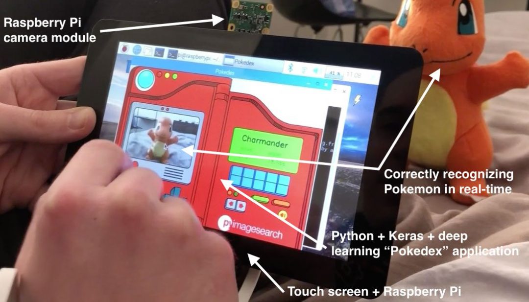
在这个系列中，我们一直在实现我儿时的梦想:建造一个 Pokedex。

Pokedex 是一个来自口袋妖怪世界的虚构设备(我过去是/现在仍然是一个超级口袋妖怪书呆子) 并允许最终用户:

1. 把它对准一个口袋妖怪(类似动物的生物)，大概是用某种相机
2. 并且自动识别口袋妖怪，提供关于该生物的详细信息

因此，你可以把 Pokedex 想象成一个智能手机应用程序，它(1)访问你的相机，并且(2)实时识别动物/生物。

为了识别口袋妖怪，我们使用 Keras 训练了一个卷积神经网络——这个模型能够正确识别图像和视频流中的口袋妖怪。

然后使用 Keras、CoreML 和 iOS 将该模型部署到移动应用程序，以创建实际的“Pokedex 应用程序”。

但是为什么要止步于此呢？

PyImageSearch 博客的长期读者都知道我喜欢树莓派…

…我情不自禁地制作了一个实际的 Pokedex 设备，使用了:

• 树莓派
• 相机模块
• 7 英寸触摸屏

这个系列肯定是一个有趣的怀旧项目——谢谢你陪我走完这段旅程。

要了解这个有趣的深度学习项目的更多信息，并在树莓 Pi 上实时运行深度学习模型，请继续阅读！

面向初学者、学生和业余爱好者的有趣的动手深度学习项目

https://www.youtube.com/embed/em1oFZO-XW8?feature=oembed

深度学习对象检测的温和指南

原文：https://pyimagesearch.com/2018/05/14/a-gentle-guide-to-deep-learning-object-detection/

今天的博客帖子是受 PyImageSearch 读者 Ezekiel 的启发，他上周给我发了一封电子邮件，问我:

嘿阿德里安，

我浏览了你之前关于深度学习对象检测和
的博文，以及实时深度学习对象检测的后续教程。谢谢你。

我一直在我的示例项目中使用您的源代码，但是我有两个问题:

1. 如何过滤/忽略我不感兴趣的课程？
2. 如何向我的对象检测器添加新的类？这可能吗？

如果你能在博客中对此进行报道，我将不胜感激。

谢了。

以西结不是唯一有这些问题的读者。事实上，如果你浏览我最近两篇关于深度学习对象检测的帖子的评论部分(链接如上)，你会发现最常见的问题之一通常是(转述):

我如何修改你的源代码来包含我自己的对象类？

由于这似乎是一个如此常见的问题，最终是对神经网络/深度学习对象检测器实际工作方式的误解，我决定在今天的博客帖子中重新讨论深度学习对象检测的话题。

具体来说，在这篇文章中，你将学到:

• 图像分类和物体检测的区别
• 深度学习对象检测器的组成包括 n 对象检测框架和基础模型本身的区别
• 如何用预训练模型进行深度学习物体检测
• 如何从深度学习模型中过滤并忽略预测类
• 在深度神经网络中添加或删除类别时的常见误解和误会

要了解更多关于深度学习对象检测的信息，甚至可能揭穿你对基于深度学习的对象检测可能存在的一些误解或误会，请继续阅读。

深度学习对象检测的温和指南

今天的博客旨在温和地介绍基于深度学习的对象检测。

我已经尽了最大努力来提供深度学习对象检测器的组件的评论，包括使用预训练的对象检测器执行深度学习的 OpenCV + Python 源代码。

使用本指南来帮助你开始深度学习对象检测，但也要认识到对象检测是高度细致入微的——我不可能在一篇博客文章中包括深度学习对象检测的每个细节。

也就是说，我们将从讨论图像分类和对象检测之间的基本差异开始今天的博客文章，包括为图像分类训练的网络是否可以用于对象检测(以及在什么情况下)。

一旦我们理解了什么是对象检测，我们将回顾深度学习对象检测器的核心组件，包括对象检测框架以及基础模型，这两个关键组件是对象检测新手容易误解的。

从那里，我们将使用 OpenCV 实现实时深度学习对象检测。

我还将演示如何忽略和过滤你不感兴趣的对象类 而不必修改网络架构或重新训练模型。

最后，我们将通过讨论如何从深度学习对象检测器添加或删除类来结束今天的博客帖子，包括我推荐的帮助您入门的资源。

让我们继续深入学习对象检测！

图像分类和目标检测的区别

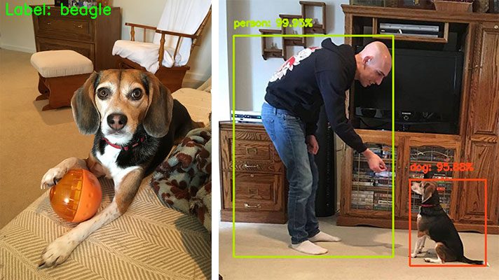
Figure 1: The difference between classification (left) and object detection (right) is intuitive and straightforward. For image classification, the entire image is classified with a single label. In the case of object detection, our neural network localizes (potentially multiple) objects within the image.

当执行标准的图像分类时，给定一个输入图像，我们将其呈现给我们的神经网络，并且我们获得一个单个类别标签，并且可能还获得与类别标签相关联的概率。

这个类标签用来描述整个图像的内容，或者至少是图像中最主要的可见内容。

例如，给定上面图 1(左)中的输入图像，我们的 CNN 将该图像标记为*【小猎犬】*。

因此我们可以把图像分类看作:

• 在中的一个图像
• 并且一个类标签出

物体检测，无论是通过深度学习还是其他计算机视觉技术执行，都建立在图像分类的基础上，并寻求准确定位每个物体在图像中出现的位置。

当执行对象检测时，给定输入图像，我们希望获得:

• 一个边界框列表，或 (x，y)-图像中每个对象的坐标
• 与每个边界框相关联的类标签
• 与每个边界框和类别标签相关联的概率/置信度得分

图 1 ( 右)演示了执行深度学习对象检测的示例。注意人和狗是如何被定位的，它们的边界框和类别标签是被预测的。

因此，物体检测使我们能够:

• 向网络展示一幅图像
• 并且获得多个包围盒和类别标签出

深度学习图像分类器可以用于物体检测吗？

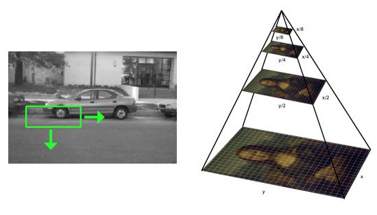
Figure 2: A non-end-to-end deep learning object detector uses a sliding window (left) + image pyramid (right) approach combined with classification.

好了，至此你明白了图像分类和物体检测之间的根本区别:

• 当执行图像分类时，我们将一幅输入图像呈现给网络，并获得一个类别标签输出。
• 但是当执行对象检测时，我们可以呈现一个输入图像并获得多个包围盒和类别标签。

这引发了一个问题:

我们能不能用一个已经训练好的网络来进行分类，然后用它来进行物体检测呢？

这个答案有点棘手，因为从技术上来说它是*“是”*，但原因并不那么明显。

解决方案包括:

1. 应用标准的基于计算机视觉的物体检测方法(即非深度学习方法)，如滑动窗口和图像金字塔——这种方法通常用于您的 HOG +基于线性 SVM 的物体检测器。
2. 取预先训练好的网络作为深度学习对象检测框架(即更快的 R-CNN、SSD、YOLO)中的基网络。

方法#1:传统的对象检测管道

第一种方法是而不是一个纯端到端的深度学习对象检测器。

相反，我们利用:

1. 固定大小的 滑动窗口 ，从左到右和从上到下滑动以定位不同位置的对象
2. 一个 图像金字塔 以不同的比例检测物体
3. 通过预训练(分类)卷积神经网络的分类

在滑动窗口+图像金字塔的每一站，我们提取 ROI，将其输入 CNN，并获得 ROI 的输出分类。

如果标签 L 的分类概率高于某个阈值 T ，我们将感兴趣区域的包围盒标记为标签( L )。对滑动窗口和图像金字塔的每次停止重复这个过程，我们获得输出对象检测器。最后，我们将非最大值抑制应用于边界框，产生我们的最终输出检测:

Figure 3: Applying non-maxima suppression will suppress overlapping, less confident bounding boxes.

这种方法可以在一些特定的用例中工作，但是一般来说它很慢，很乏味，并且有点容易出错。

然而，值得学习如何应用这种方法，因为它可以将任意图像分类网络变成对象检测器，*避免了显式训练端到端深度学习对象检测器的需要。*根据您的使用情况，这种方法可以节省您大量的时间和精力。

如果你对这种物体检测方法感兴趣，并想了解更多关于滑动窗口+图像金字塔+图像分类的物体检测方法，请参考我的书， 用 Python 进行计算机视觉的深度学习 。

方法#2:对象检测框架的基础网络

深度学习对象检测的第二种方法允许你将你预先训练的分类网络视为一个深度学习对象检测框架中的基础网络(例如更快的 R-CNN、SSD 或 YOLO)。

这里的好处是，你可以创建一个完整的端到端的基于深度学习的对象检测器。

缺点是，它需要一些关于深度学习对象检测器如何工作的深入知识——我们将在下一节中对此进行更多讨论。

深度学习对象检测器的组件

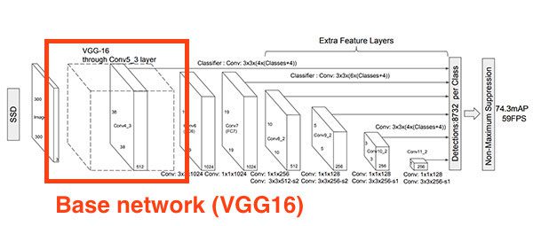
Figure 4: The VGG16 base network is a component of the SSD deep learning object detection framework.

深度学习对象检测器有许多组件、子组件和子子组件，但我们今天要关注的两个是大多数深度学习对象检测新手经常混淆的两个组件:

1. 对象检测框架(例如。更快的 R-CNN，SSD，YOLO)。
2. 适合目标检测框架的基础网络。

你可能已经熟悉的基础网络(你只是以前没有听说过它被称为“基础网络”)。

基本网络是您常见的(分类)CNN 架构，包括:

• VGGNet
• ResNet
• MobileNet
• DenseNet

通常，这些网络经过预先训练，可以在大型图像数据集(如 ImageNet)上执行分类，以学习一组丰富的辨别、鉴别过滤器。

对象检测框架由许多组件和子组件组成。

例如，更快的 R-CNN 框架包括:

• 区域提案网络
• 一套锚
• 感兴趣区域(ROI)汇集模块
• 最终基于区域的卷积神经网络

使用**单触发探测器(SSD)**时，您有组件和子组件，例如:

• 多框
• 传道者
• 固定前科

请记住，基础网络只是适合整体深度学习对象检测框架的众多组件之一——本节顶部的图 4 描绘了 SSD 框架内的 VGG16 基础网络。

通常，“网络手术”是在基础网络上进行的。这一修改:

• 形成完全卷积(即，接受任意输入维度)。
• 消除基础网络架构中更深层的 conv/池层，代之以一系列新层(SSD)、新模块(更快的 R-CNN)或两者的某种组合。

术语“网络手术”是一种通俗的说法，意思是我们移除基础网络架构中的一些原始层，并用新层取而代之。

你可能看过一些低成本的恐怖电影，在这些电影中，凶手可能拿着一把斧头或大刀，袭击受害者，并毫不客气地攻击他们。

网络手术比典型的 B 级恐怖片杀手更加精确和苛刻。

网络手术也是战术性的——我们移除网络中我们不需要的部分，并用一组新的组件替换它。

然后，当我们去训练我们的框架来执行对象检测时，修改(1)新的层/模块和(2)基础网络的权重。

同样，对各种深度学习对象检测框架如何工作(包括基础网络扮演的角色)的完整回顾不在这篇博文的范围之内。

如果你对深度学习对象检测的完整回顾感兴趣，包括理论和实现，请参考我的书， 用 Python 进行计算机视觉的深度学习 。

我如何衡量深度学习对象检测器的准确性？

在评估对象检测器性能时，我们使用一个名为平均精度 (mAP)的评估指标，该指标基于我们数据集中所有类的 交集与 (IoU)。

并集上的交集

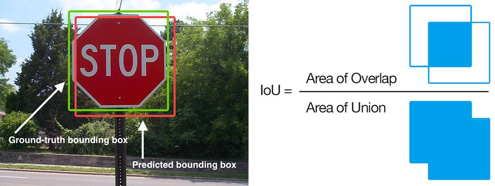
Figure 5: In this visual example of Intersection over Union (IoU), the ground-truth bounding box (green) can be compared to the predicted bounding box (red). IoU is used with mean Average Precision (mAP) to evaluate the accuracy of a deep learning object detector. The simple equation to calculate IoU is shown on the right.

您通常会发现 IoU 和 mAP 用于评估 HOG +线性 SVM 检测器、Haar 级联和基于深度学习的方法的性能；但是，请记住，用于生成预测边界框的实际算法并不重要。

任何提供预测边界框(以及可选的类标签)作为输出的算法都可以使用 IoU 进行评估。更正式地说，为了应用 IoU 来评估任意对象检测器，我们需要:

1. 真实边界框(即，我们的测试集中的手绘边界框，它指定了我们的对象在图像中的位置)。
2. 我们模型中的预测边界框。
3. 如果您想计算召回率和精确度，您还需要基本事实类标签和预测类标签。

在图 5 ( 左)中，我包含了一个真实边界框(绿色)与预测边界框(红色)的可视化示例。计算 IoU 可以通过图 5 ( 右)中的等式图示来确定。

检查这个等式，你会发现, IoU 仅仅是一个比率。

在分子中，我们计算预测边界框和真实边界框之间的重叠区域。

分母是并集的面积，或者更简单地说，是由预测边界框和实际边界框包围的面积。

将重叠面积除以并集面积得到最终分数，即并集上的交集。

平均精度

***注:*我决定编辑这一节的原貌。我想让对地图的讨论保持在更高的水平，避免一些更令人困惑的回忆计算，但正如一些评论者指出的，这一部分在技术上是不正确的。因此，我决定更新帖子。

因为这是对基于深度学习的对象检测的温和介绍，所以我将保持对 mAP 的简化解释，以便您理解基本原理。

不熟悉对象检测的读者和从业者可能会被地图计算弄糊涂。这部分是因为 mAP 是一个更复杂的评估指标。它也是 mAP 计算的定义，甚至可以从一个对象检测挑战变化到另一个(当我说“对象检测挑战”时，我指的是诸如 COCO、PASCAL VOC 等竞赛。).

计算特定对象检测流水线的平均精度(AP)基本上是一个三步过程:

1. 计算精度，它是真阳性的比例。
2. 计算召回，这是所有可能的阳性中真正阳性的比例。
3. 以 s. 为步长，对所有召回级别的最大精度值进行平均

为了计算精度，我们首先将我们的对象检测算法应用于输入图像。然后，边界框分数按照置信度降序排列。

我们从先验知识中得知(即，这是一个验证/测试示例，因此我们知道图像中对象的总数)该图像中有 4 个对象。我们试图确定我们的网络进行了多少次“正确的”检测。这里的“正确”预测是指 IoU 最小值为 0.5(该值可根据挑战进行调整，但 0.5 是标准值)。

这就是计算开始变得有点复杂的地方。我们需要计算不同召回值(也称为“召回级别”或“召回步骤”)的精确度。

例如，假设我们正在计算前 3 个预测的精度和召回值。在深度学习对象检测器的前 3 个预测中，我们做出了 2 个正确的预测。那么我们的精度就是真阳性的比例:2/3 = 0.667。我们的回忆是图像中所有可能的阳性中真正的阳性的比例:2 / 4 = 0.5。我们对(通常)前 1 到前 10 个预测重复这个过程。这个过程产生一个精度值的列表。

下一步是计算所有 top- N 值的平均值，因此有术语平均精度(AP) 。我们循环所有的召回值 r ，找到我们可以用召回值r获得的最大精度 p ，然后计算平均值。我们现在有了单个评估图像的平均精度。

一旦我们计算了测试/验证集中所有图像的平均精度，我们将执行另外两个计算:

1. 计算每个类别的平均 AP，为每个单独的类别提供一个地图(对于许多数据集/挑战，您将需要按类别检查地图，以便您可以发现您的深度学习对象检测器是否正在处理特定的类别)
2. 获取每个单独类的地图，然后将它们平均在一起，得到数据集的最终地图

同样，地图比传统的准确性更复杂，所以如果你第一次看不懂也不要沮丧。这是一个评估指标，在你完全理解它之前，你需要多次研究。好消息是深度学习对象检测实现为你处理计算地图。

基于深度学习的 OpenCV 物体检测

在之前的帖子中，我们已经在这个博客上讨论了深度学习和对象检测；然而，为了完整起见，让我们回顾一下本帖中的实际源代码。

我们的示例包括带有 MobileNet 基本模型的单次检测器(框架)。该模型由 GitHub 用户 chuanqi305 在上下文通用对象(COCO)数据集上进行训练。

要了解更多细节，请查看我的 上一篇文章 ，在那里我介绍了传祺 305 的模型和相关的背景信息。

让我们从这篇文章的顶部回到以西结的第一个问题:

1. How do I filter/ignore classes that I am not interested in?

我将在下面的示例脚本中回答这个问题。

但是首先你需要准备你的系统:

• 您需要在您的 Python 虚拟环境中安装最低的 OpenCV 3.3(假设您使用的是 Python 虚拟环境)。OpenCV 3.3+包括运行以下代码所需的 DNN 模块。确保使用下页的 OpenCV 安装教程，同时特别注意你下载并安装的是哪个版本的 OpenCV。
• 你也应该安装我的 imutils 包。要在 Python 虚拟环境中安装/更新 imutils，只需使用 pip: pip install --upgrade imutils。

当你准备好了，继续创建一个名为filter_object_detection.py的新文件，让我们开始吧:

# import the necessary packages
from imutils.video import VideoStream
from imutils.video import FPS
import numpy as np
import argparse
import imutils
import time
import cv2

在的第 2-8 行，我们导入我们需要的包和模块，特别是imutils和 OpenCV。我们将使用我的VideoStream类来处理从网络摄像头捕捉帧。

我们配备了必要的工具，所以让我们继续解析命令行参数:

# construct the argument parse and parse the arguments
ap = argparse.ArgumentParser()
ap.add_argument("-p", "--prototxt", required=True,
	help="path to Caffe 'deploy' prototxt file")
ap.add_argument("-m", "--model", required=True,
	help="path to Caffe pre-trained model")
ap.add_argument("-c", "--confidence", type=float, default=0.2,
	help="minimum probability to filter weak detections")
args = vars(ap.parse_args())

我们的脚本在运行时需要两个命令行参数:

• --prototxt:定义模型定义的 Caffe prototxt 文件的路径。
• --model:我们的 CNN 模型权重文件路径。

您可以选择指定一个阈值--confidence，用于过滤弱检测。

我们的模型可以预测 21 个对象类别:

# initialize the list of class labels MobileNet SSD was trained to
# detect, then generate a set of bounding box colors for each class
CLASSES = ["background", "aeroplane", "bicycle", "bird", "boat",
	"bottle", "bus", "car", "cat", "chair", "cow", "diningtable",
	"dog", "horse", "motorbike", "person", "pottedplant", "sheep",
	"sofa", "train", "tvmonitor"]

CLASSES列表包含网络被训练的所有类别标签(即 COCO 标签)。

对CLASSES列表的一个常见误解是，您可以:

1. 向列表中添加一个新的类别标签
2. 或者从列表中删除一个类别标签

…让网络自动“知道”您想要完成的任务。

事实并非如此。

你不能简单地修改一列文本标签，让网络自动修改自己，以学习、添加或删除它从未训练过的数据模式。这不是神经网络的工作方式。

也就是说，有一个快速技巧可以用来过滤和忽略你不感兴趣的预测。

解决方案是:

1. 定义一组IGNORE标签(即训练网络时要过滤和忽略的类别标签列表)。
2. 对输入图像/视频帧进行预测。
3. 忽略类别标签存在于IGNORE集合中的任何预测。

用 Python 实现的IGNORE集合如下所示:

IGNORE = set(["person"])

这里我们将忽略所有带有类标签"person"的预测对象(用于过滤的if语句将在后面的代码审查中讨论)。

您可以轻松地向集合中添加要忽略的附加元素(来自CLASSES列表的类标签)。

接下来，我们将生成随机标签/盒子颜色，加载我们的模型，并开始视频流:

COLORS = np.random.uniform(0, 255, size=(len(CLASSES), 3))

# load our serialized model from disk
print("[INFO] loading model...")
net = cv2.dnn.readNetFromCaffe(args["prototxt"], args["model"])

# initialize the video stream, allow the cammera sensor to warmup,
# and initialize the FPS counter
print("[INFO] starting video stream...")
vs = VideoStream(src=0).start()
time.sleep(2.0)
fps = FPS().start()

在线 27 上，生成随机数组COLORS以对应 21 个CLASSES中的每一个。我们稍后将使用这些颜色进行显示。

我们的 Caffe 模型通过使用cv2.dnn.readNetFromCaffe函数和作为参数传递的两个必需的命令行参数在行 31 上加载。

然后我们将VideoStream对象实例化为vs，并启动我们的fps计数器(第 36-38 行)。2 秒钟的sleep让我们的相机有足够的时间预热。

在这一点上，我们准备好循环从摄像机传入的帧，并通过我们的 CNN 对象检测器发送它们:

# loop over the frames from the video stream
while True:
	# grab the frame from the threaded video stream and resize it
	# to have a maximum width of 400 pixels
	frame = vs.read()
	frame = imutils.resize(frame, width=400)

	# grab the frame dimensions and convert it to a blob
	(h, w) = frame.shape[:2]
	blob = cv2.dnn.blobFromImage(cv2.resize(frame, (300, 300)),
		0.007843, (300, 300), 127.5)

	# pass the blob through the network and obtain the detections and
	# predictions
	net.setInput(blob)
	detections = net.forward()

在第 44 行上，我们抓取一个frame然后resize，同时保留显示的纵横比(第 45 行)。

从那里，我们提取高度和宽度，因为我们稍后需要这些值( Line 48 )。

第 48 和 49 行从我们的帧生成一个blob。要了解更多关于一个blob以及如何使用cv2.dnn.blobFromImage函数构造它的信息，请参考上一篇文章了解所有细节。

接下来，我们通过我们的神经net发送那个blob来检测物体(线 54 和 55 )。

让我们循环一下检测结果:

	# loop over the detections
	for i in np.arange(0, detections.shape[2]):
		# extract the confidence (i.e., probability) associated with
		# the prediction
		confidence = detections[0, 0, i, 2]

		# filter out weak detections by ensuring the `confidence` is
		# greater than the minimum confidence
		if confidence > args["confidence"]:
			# extract the index of the class label from the
			# `detections`
			idx = int(detections[0, 0, i, 1])

			# if the predicted class label is in the set of classes
			# we want to ignore then skip the detection
			if CLASSES[idx] in IGNORE:
				continue

在第 58 条线上，我们开始了我们的detections循环。

对于每个检测，我们提取confidence ( 行 61 )，然后将其与我们的置信度阈值(行 65 )进行比较。

在我们的confidence超过最小值的情况下(默认值 0.2 可以通过可选的命令行参数来更改)，我们将认为检测是积极的、有效的检测，并继续处理它。

首先，我们从detections ( 第 68 行)中提取类标签的索引。

然后，回到以西结的第一个问题，我们可以忽略第 72 行和第 73 行的IGNORE集合中的类。如果要忽略该类，我们只需continue返回到检测循环的顶部(并且我们不显示该类的标签或框)。这实现了我们的“快速破解”解决方案。

否则，我们在白名单中检测到一个对象，我们需要在框架上显示类别标签和矩形:

			# compute the (x, y)-coordinates of the bounding box for
			# the object
			box = detections[0, 0, i, 3:7] * np.array([w, h, w, h])
			(startX, startY, endX, endY) = box.astype("int")

			# draw the prediction on the frame
			label = "{}: {:.2f}%".format(CLASSES[idx],
				confidence * 100)
			cv2.rectangle(frame, (startX, startY), (endX, endY),
				COLORS[idx], 2)
			y = startY - 15 if startY - 15 > 15 else startY + 15
			cv2.putText(frame, label, (startX, y),
				cv2.FONT_HERSHEY_SIMPLEX, 0.5, COLORS[idx], 2)

在这个代码块中，我们提取边界框坐标(行 77 和 78 )，然后在框架上绘制一个标签和矩形(行 81-87 )。

对于每个唯一的类，标签+矩形的颜色将是相同的；相同类别的对象将具有相同的颜色(即视频中的所有"boats"将具有相同的颜色标签和框)。

最后，仍在我们的while循环中，我们将在屏幕上显示我们的辛勤工作:

	# show the output frame
	cv2.imshow("Frame", frame)
	key = cv2.waitKey(1) & 0xFF

	# if the `q` key was pressed, break from the loop
	if key == ord("q"):
		break

	# update the FPS counter
	fps.update()

# stop the timer and display FPS information
fps.stop()
print("[INFO] elapsed time: {:.2f}".format(fps.elapsed()))
print("[INFO] approx. FPS: {:.2f}".format(fps.fps()))

# do a bit of cleanup
cv2.destroyAllWindows()
vs.stop()

我们在第 90 和 91 行上显示frame并捕捉按键。

如果按下"q"键，我们通过中断循环退出(行 94 和 95 )。

否则，我们继续更新我们的fps计数器(行 98 )并继续抓取和处理帧。

在剩余的行中，当循环中断时，我们显示时间+每秒帧数指标和清理。

运行深度学习对象检测器

为了运行今天的脚本，您需要通过滚动到下面的 【下载】 部分来获取文件。

提取文件后，打开终端并导航到下载的代码+模型。在那里，执行以下命令:

$ python filter_object_detection.py --prototxt MobileNetSSD_deploy.prototxt.txt \
	--model MobileNetSSD_deploy.caffemodel
[INFO] loading model...
[INFO] starting video stream...
[INFO] elapsed time: 24.05
[INFO] approx. FPS: 13.18

Figure 6: A real-time deep learning object detection demonstration of using the same model — in the right video I’ve ignored certain object classes programmatically.

在上面的 GIF 中，你可以看到在的左边检测到了*“人”类——这是因为我有一个空的IGNORE。在右边的中您可以看到我没有被检测到——这种行为是由于将“person”*类添加到了IGNORE集合中。

当我们的深度学习对象检测器仍然在技术上检测*“person”*类时，我们的后处理代码能够将其过滤掉。

也许你在运行深度学习对象检测器时遇到了错误？

故障诊断的第一步是验证您是否连接了网络摄像头。如果这不是问题所在，您可能会在终端中看到以下错误消息:

$ python filter_object_detection.py 
usage: filter_object_detection.py [-h] -p PROTOTXT -m MODEL [-c CONFIDENCE]
filter_object_detection.py: error: the following arguments are required: -p/--prototxt, -m/--model

如果你看到这个消息，那么你没有传递“命令行参数”给程序。如果 PyImageSearch 读者不熟悉 Python、argparse 和命令行参数 ，这是一个常见问题。如果你有问题，请查看链接。

以下是带评论的完整视频:

https://www.youtube.com/embed/5cwFBUQb6_w?feature=oembed