PyImgSearch 博客中文翻译（七）

原文：PyImgSearch Blog

协议：CC BY-NC-SA 4.0

使用 Python 将深度学习和 RBM 应用于 MNIST

原文：https://pyimagesearch.com/2014/06/23/applying-deep-learning-rbm-mnist-using-python/

在我的上一篇文章中，我提到过，当利用原始像素作为特征向量时，图像中微小的一个像素偏移会破坏受限的玻尔兹曼机器+分类器流水线的性能。

今天我将继续这一讨论。

更重要的是，我将提供一些 Python 和 scikit-learn 代码，你可以使用这些代码来将受限的波尔兹曼机器应用到你自己的图像分类问题中。

OpenCV 和 Python 版本:
这个例子将运行在 Python 2.7 和 OpenCV 2.4.X/OpenCV 3.0+ 上。

但是在我们进入代码之前，让我们花点时间来讨论一下 MNIST 数据集。

MNIST 数据集

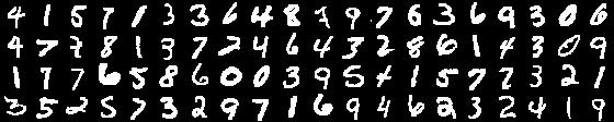
Figure 1: MNIST digit recognition sample

MNIST 数据集是计算机视觉和机器学习文献中研究得最多的数据集之一。在许多情况下，它是一个基准，一些机器学习算法的排名标准。

这个数据集的目标是正确分类手写数字 0-9。我们不打算利用整个数据集(由 60，000 幅训练图像和 10，000 幅测试图像组成)，而是利用一个小样本(3，000 幅用于训练，2，000 幅用于测试)。每个数字的数据点大致均匀分布，因此不存在明显的类别标签不平衡。

每个特征向量是 784-dim，对应于图像的28×28灰度像素强度。这些灰度像素强度是无符号整数，范围在[0，255]内。

所有数字都放在黑色背景上，前景是白色和灰色阴影。

给定这些原始像素强度，我们将首先根据我们的训练数据训练一个受限的玻尔兹曼机器，以学习数字的无监督特征表示。

然后，我们将采用这些“学习”的特征，并在它们的基础上训练一个逻辑回归分类器。

为了评估我们的管道，我们将获取测试数据，并通过我们的分类器运行它，并报告准确性。

然而，我在之前的帖子中提到，测试集图像简单的一个像素平移会导致精度下降，即使这些平移小到人眼几乎察觉不到(如果有的话)。

为了测试这种说法，我们将通过将每幅图像向上、向下、向左和向右平移一个像素来生成一个比原始图像大四倍的测试集。

最后，我们将通过管道传递这个“轻推”数据集，并报告我们的结果。

听起来不错吧？

让我们检查一些代码。

使用 Python 将 RBM 应用于 MNIST 数据集

我们要做的第一件事是创建一个文件rbm.py，并开始导入我们需要的包:

# import the necessary packages
from sklearn.cross_validation import train_test_split
from sklearn.metrics import classification_report
from sklearn.linear_model import LogisticRegression
from sklearn.neural_network import BernoulliRBM
from sklearn.grid_search import GridSearchCV
from sklearn.pipeline import Pipeline
import numpy as np
import argparse
import time
import cv2

我们将从导入 scikit-learn 的cross_validation子包中的train_test_split函数开始。train_test_split函数将使我们创建 MNIST 数据集的训练和测试分割变得非常简单。

接下来，我们将从metrics子包中导入classification_report函数，我们将使用它来生成一个关于(1)整个系统和(2)每个单独类标签的精度的格式良好的精度报告。

在第 4 行的上，我们将导入我们将在整个例子中使用的分类器——一个LogisticRegression分类器。

我提到过，我们将使用受限玻尔兹曼机器来学习原始像素值的无监督表示。这将由 scikit-learn 的neural_network子包中的BernoulliRBM类来处理。

BernoulliRBM实现(顾名思义)，由二进制可见单元和二进制隐藏节点组成。算法本身是 O(d² ) ，其中 d 是需要学习的元件个数。

为了找到逻辑回归系数C的最佳值，以及我们的 RBM 的最佳学习速率、迭代次数和组件数量，我们需要在特征空间上执行交叉验证网格搜索。GridSearchCV类(我们在6 号线上导入的)将为我们处理这个搜索。

接下来，我们需要在行 7 导入的Pipeline类。这个类允许我们使用 scikit-learn 估计器的拟合和转换方法来定义一系列步骤。

我们的分类管道将包括首先训练一个BernoulliRBM来学习特征空间的无监督表示，然后在学习的特征上训练一个LogisticRegression分类器。

最后，我们导入 NumPy 进行数值处理，argparse解析命令行参数，time跟踪给定模型训练所需的时间，而cv2用于 OpenCV 绑定。

但是在我们开始之前，我们首先需要设置一些函数来加载和操作我们的 MNIST 数据集:

def load_digits(datasetPath):
	# build the dataset and then split it into data
	# and labels
	X = np.genfromtxt(datasetPath, delimiter = ",", dtype = "uint8")
	y = X[:, 0]
	X = X[:, 1:]

	# return a tuple of the data and targets
	return (X, y)

load_digits函数，顾名思义，从磁盘上加载我们的 MNIST 数字数据集。该函数采用一个参数datasetPath，它是数据集 CSV 文件所在的路径。

我们使用np.genfromtxt函数从磁盘上加载 CSV 文件，在行 17 上抓取类标签(这是 CSV 文件的第一列)，然后在行 18 上抓取实际的原始像素特征向量。这些特征向量是 784 维的，对应于灰度数字图像的28×28展平表示。

最后，我们在第 21 行的上返回我们的特征向量矩阵和类标签的元组。

接下来，我们需要一个函数对我们的数据进行一些预处理。

BernoulliRBM假设我们的特征向量的列落在范围[0，1]内。但是，MNIST 数据集表示为无符号的 8 位整数，范围在[0，255]内。

为了将列缩放到范围[0，1]，我们需要做的就是定义一个scale函数:

def scale(X, eps = 0.001):
	# scale the data points s.t the columns of the feature space
	# (i.e the predictors) are within the range [0, 1]
	return (X - np.min(X, axis = 0)) / (np.max(X, axis = 0) + eps)

scale函数有两个参数，我们的数据矩阵X和一个用于防止被零除错误的 epsilon 值。

这个函数是不言自明的。对于矩阵中 784 列中的每一列，我们从该列的最小值中减去该值，然后除以该列的最大值。通过这样做，我们确保了每一列的值都在范围[0，1]内。

现在我们需要最后一个函数:一个生成比原始数据集大四倍的“轻推”数据集的方法，将每张图像向上、向下、向左和向右平移一个像素。

为了处理数据集的这种微调，我们将创建nudge函数:

def nudge(X, y):
	# initialize the translations to shift the image one pixel
	# up, down, left, and right, then initialize the new data
	# matrix and targets
	translations = [(0, -1), (0, 1), (-1, 0), (1, 0)]
	data = []
	target = []

	# loop over each of the digits
	for (image, label) in zip(X, y):
		# reshape the image from a feature vector of 784 raw
		# pixel intensities to a 28x28 'image'
		image = image.reshape(28, 28)

		# loop over the translations
		for (tX, tY) in translations:
			# translate the image
			M = np.float32([[1, 0, tX], [0, 1, tY]])
			trans = cv2.warpAffine(image, M, (28, 28))

			# update the list of data and target
			data.append(trans.flatten())
			target.append(label)

	# return a tuple of the data matrix and targets
	return (np.array(data), np.array(target))

nudge函数有两个参数:我们的数据矩阵X和我们的类标签y。

我们首先初始化一个(x，y) translations列表，然后是新的data矩阵和第 32-34 行的标签。

然后，我们开始遍历Line 37上的每个图像和类标签。

正如我提到的，每个图像都被表示为一个 784 维的特征向量，对应于 28 x 28 数字图像。

然而，为了利用cv2.warpAffine函数来翻译我们的图像，我们首先需要将 784 特征向量重新整形为一个形状为(28, 28)的二维数组——这是在行 40 上处理的。

接下来，我们开始在第 43 条线上的translations上循环。

我们在行 45 上构建我们实际的翻译矩阵M，然后通过调用行 46 上的cv2.warpAffine函数来应用翻译。

然后，我们能够通过将 28 x 28 图像展平回 784-dim 特征向量来更新行 48 上的新的微推data矩阵。

我们的类标签target列表随后在行的第 50 处被更新。

最后，我们在第 53 行的返回新数据矩阵和类标签的元组。

这三个辅助函数虽然本质上很简单，但对于设置我们的实验却至关重要。

现在我们终于可以开始把这些碎片拼在一起了:

# construct the argument parser and parse the arguments
ap = argparse.ArgumentParser()
ap.add_argument("-d", "--dataset", required = True,
	help = "path to the dataset file")
ap.add_argument("-t", "--test", required = True, type = float,
	help = "size of test split")
ap.add_argument("-s", "--search", type = int, default = 0,
	help = "whether or not a grid search should be performed")
args = vars(ap.parse_args())

第 56-63 行处理解析我们的命令行参数。我们的rbm.py脚本需要三个参数:--dataset，这是我们的 MNIST 所在的路径。csv 文件驻留在磁盘上，--test，用于我们的测试分割的数据百分比(其余用于训练)，以及--search，一个用于确定是否应该执行网格搜索来调整超参数的整数。

--search的值1表示应该执行网格搜索；值0表示已经进行了网格搜索，并且已经手动设置了BernoulliRBM和LogisticRegression模型的模型参数。

# load the digits dataset, convert the data points from integers
# to floats, and then scale the data s.t. the predictors (columns)
# are within the range [0, 1] -- this is a requirement of the
# Bernoulli RBM
(X, y) = load_digits(args["dataset"])
X = X.astype("float32")
X = scale(X)

# construct the training/testing split
(trainX, testX, trainY, testY) = train_test_split(X, y,
	test_size = args["test"], random_state = 42)

现在我们的命令行参数已经被解析了，我们可以在第 69 行的上从磁盘上加载我们的数据集。然后我们在行 70** 上将其转换为浮点数据类型，并使用行 71 上的scale函数将特征向量列缩放到范围[0，1]内。**

为了评估我们的系统，我们需要两组数据:训练集和测试集。我们的管道将使用训练数据进行训练，然后使用测试集进行评估，以确保我们的准确性报告不会有偏差。

为了生成我们的训练和测试分割，我们将调用第 74 行上的train_test_split函数。这个函数会自动为我们生成拆分。

# check to see if a grid search should be done
if args["search"] == 1:
	# perform a grid search on the 'C' parameter of Logistic
	# Regression
	print "SEARCHING LOGISTIC REGRESSION"
	params = {
    
    "C": [1.0, 10.0, 100.0]}
	start = time.time()
	gs = GridSearchCV(LogisticRegression(), params, n_jobs = -1, verbose = 1)
	gs.fit(trainX, trainY)

	# print diagnostic information to the user and grab the
	# best model
	print "done in %0.3fs" % (time.time() - start)
	print "best score: %0.3f" % (gs.best_score_)
	print "LOGISTIC REGRESSION PARAMETERS"
	bestParams = gs.best_estimator_.get_params()

	# loop over the parameters and print each of them out
	# so they can be manually set
	for p in sorted(params.keys()):
		print "\t %s: %f" % (p, bestParams[p])

在行 78 上进行检查，以查看是否应该执行网格搜索来调整我们管道的超参数。

如果要执行网格搜索，我们首先在第 81-85 行上搜索逻辑回归分类器的系数C。我们将对原始像素数据 和 仅使用逻辑回归分类器来评估我们的方法，受限的波尔兹曼机器+逻辑回归分类器，因此我们需要独立地搜索系数C空间。

第 89-97 行然后打印出标准逻辑回归分类器的最佳参数值。

现在我们可以继续我们的管道:一个BernoulliRBM和一个LogisticRegression分类器一起使用。

	# initialize the RBM + Logistic Regression pipeline
	rbm = BernoulliRBM()
	logistic = LogisticRegression()
	classifier = Pipeline([("rbm", rbm), ("logistic", logistic)])

	# perform a grid search on the learning rate, number of
	# iterations, and number of components on the RBM and
	# C for Logistic Regression
	print "SEARCHING RBM + LOGISTIC REGRESSION"
	params = {
    
    
		"rbm__learning_rate": [0.1, 0.01, 0.001],
		"rbm__n_iter": [20, 40, 80],
		"rbm__n_components": [50, 100, 200],
		"logistic__C": [1.0, 10.0, 100.0]}

	# perform a grid search over the parameter
	start = time.time()
	gs = GridSearchCV(classifier, params, n_jobs = -1, verbose = 1)
	gs.fit(trainX, trainY)

	# print diagnostic information to the user and grab the
	# best model
	print "\ndone in %0.3fs" % (time.time() - start)
	print "best score: %0.3f" % (gs.best_score_)
	print "RBM + LOGISTIC REGRESSION PARAMETERS"
	bestParams = gs.best_estimator_.get_params()

	# loop over the parameters and print each of them out
	# so they can be manually set
	for p in sorted(params.keys()):
		print "\t %s: %f" % (p, bestParams[p])

	# show a reminder message
	print "\nIMPORTANT"
	print "Now that your parameters have been searched, manually set"
	print "them and re-run this script with --search 0"

我们在行 100-102 上定义我们的流水线，由我们的受限波尔兹曼机器和逻辑回归分类器组成。

然而，现在我们有更多的参数可以搜索，而不仅仅是逻辑回归分类器的系数C。现在，我们还必须搜索迭代次数、组件数量(即所得特征空间的大小)，以及 RBM 的学习速率。我们在第 108-112 行中定义了这个搜索空间。

我们从第 115-117 行的开始网格搜索。

然后在行 121-129 显示管道的最佳参数。

要确定管道的最佳值，请执行以下命令:

$ python rbm.py --dataset data/digits.csv --test 0.4 --search 1

在搜索网格空间时，您可能想泡一杯咖啡或者出去散散步。对于我们选择的每一个参数，都需要对模型进行训练和交叉验证。肯定不是快速操作。但这是你为最佳参数所付出的代价，当使用受限玻尔兹曼机时，这是至关重要的。

走了很长一段路后，您应该看到已经选择了以下最佳值:

rbm__learning_rate: 0.01
rbm__n_iter: 40
rbm__n_components: 200
logistic__C: 1.0

太棒了。我们的超参数已经调整好了。

让我们设置这些参数并评估我们的分类管道:

# otherwise, use the manually specified parameters
else:
	# evaluate using Logistic Regression and only the raw pixel
	# features (these parameters were cross-validated)
	logistic = LogisticRegression(C = 1.0)
	logistic.fit(trainX, trainY)
	print "LOGISTIC REGRESSION ON ORIGINAL DATASET"
	print classification_report(testY, logistic.predict(testX))

	# initialize the RBM + Logistic Regression classifier with
	# the cross-validated parameters
	rbm = BernoulliRBM(n_components = 200, n_iter = 40,
		learning_rate = 0.01,  verbose = True)
	logistic = LogisticRegression(C = 1.0)

	# train the classifier and show an evaluation report
	classifier = Pipeline([("rbm", rbm), ("logistic", logistic)])
	classifier.fit(trainX, trainY)
	print "RBM + LOGISTIC REGRESSION ON ORIGINAL DATASET"
	print classification_report(testY, classifier.predict(testX))

	# nudge the dataset and then re-evaluate
	print "RBM + LOGISTIC REGRESSION ON NUDGED DATASET"
	(testX, testY) = nudge(testX, testY)
	print classification_report(testY, classifier.predict(testX))

为了获得基线精度，我们将在第行第 140 和 141 的原始像素特征向量上训练一个标准的逻辑回归分类器(无监督学习)。然后使用classification_report功能在行 143 上打印出基线的精度。

然后，我们构建我们的BernoulliRBM + LogisticRegression分类器流水线，并在行 147-155 的测试数据上对其进行评估。

但是，当我们通过将每张图片向上、向下、向左和向右平移一个像素来微调测试集时，会发生什么呢？

为了找到答案，我们在第 162 行的处挪动数据集，然后在第 163 行的处重新评估它。

要评估我们的系统，发出以下命令:

$ python rbm.py --dataset data/digits.csv --test 0.4

几分钟后，我们应该会看到一些结果。

结果

第一组结果是我们在原始像素特征向量上严格训练的逻辑回归分类器:

LOGISTIC REGRESSION ON ORIGINAL DATASET
             precision    recall  f1-score   support

          0       0.94      0.96      0.95       196
          1       0.94      0.97      0.95       245
          2       0.89      0.90      0.90       197
          3       0.88      0.84      0.86       202
          4       0.90      0.93      0.91       193
          5       0.85      0.75      0.80       183
          6       0.91      0.93      0.92       194
          7       0.90      0.90      0.90       212
          8       0.85      0.83      0.84       186
          9       0.81      0.84      0.83       192

avg / total       0.89      0.89      0.89      2000

使用这种方法，我们能够达到 89%的准确率。使用像素亮度作为我们的特征向量并不坏。

但是看看当我们训练我们的受限玻尔兹曼机+逻辑回归流水线时会发生什么:

RBM + LOGISTIC REGRESSION ON ORIGINAL DATASET
             precision    recall  f1-score   support

          0       0.95      0.98      0.97       196
          1       0.97      0.96      0.97       245
          2       0.92      0.95      0.94       197
          3       0.93      0.91      0.92       202
          4       0.92      0.95      0.94       193
          5       0.95      0.86      0.90       183
          6       0.95      0.95      0.95       194
          7       0.93      0.91      0.92       212
          8       0.91      0.90      0.91       186
          9       0.86      0.90      0.88       192

avg / total       0.93      0.93      0.93      2000

我们的准确率能够从 89%提高到 93%！这绝对是一个重大的飞跃！

但是现在问题开始了…

当我们轻推数据集，将每幅图像向上、向下、向左和向右平移一个像素时，会发生什么？

我的意思是，这些变化是如此之小，以至于肉眼几乎无法识别。

这当然不成问题，是吗？

事实证明，是这样的:

RBM + LOGISTIC REGRESSION ON NUDGED DATASET
             precision    recall  f1-score   support

          0       0.94      0.93      0.94       784
          1       0.96      0.89      0.93       980
          2       0.87      0.91      0.89       788
          3       0.85      0.85      0.85       808
          4       0.88      0.92      0.90       772
          5       0.86      0.80      0.83       732
          6       0.90      0.91      0.90       776
          7       0.86      0.90      0.88       848
          8       0.80      0.85      0.82       744
          9       0.84      0.79      0.81       768

avg / total       0.88      0.88      0.88      8000

在轻推我们的数据集后，RBM +逻辑回归管道下降到 88%的准确率。比原始测试集低 5%，比基线逻辑回归分类器低 1%。

所以现在你可以看到使用原始像素亮度作为特征向量的问题。即使是图像中微小的偏移也会导致精确度下降。

但别担心，有办法解决这个问题。

我们如何解决翻译问题？

神经网络、深度网络和卷积网络中的研究人员有两种方法来解决移位和翻译问题。

第一种方法是在训练时生成额外的数据。

在这篇文章中，我们在训练后轻推了一下我们的数据集*,看看它对分类准确度的影响。然而，我们也可以在训练之前微调我们的数据集，试图让我们的模型更加健壮。*

第二种方法是从我们的训练图像中随机选择区域，而不是完整地使用它们。

例如，我们可以从图像中随机抽取一个 24 x 24 区域，而不是使用整个 28 x 28 图像。做足够多的次数，足够多的训练图像，我们可以减轻翻译问题。

摘要

在这篇博文中，我们已经证明了，即使是人眼几乎无法分辨的图像中微小的一个像素的平移也会损害我们的分类管道的性能。

我们看到精确度下降的原因是因为我们利用原始像素强度作为特征向量。

此外，当利用原始像素强度作为特征时，平移不是唯一会导致精度损失的变形。捕获图像时的旋转、变换甚至噪声都会对模型性能产生负面影响。

为了处理这些情况，我们可以(1)生成额外的训练数据，以尝试使我们的模型更加健壮，和/或(2)从图像中随机采样，而不是完整地使用它。

在实践中，神经网络和深度学习方法比这个实验要稳健得多。通过堆叠层和学习一组卷积核，深度网络能够处理许多这些问题。

不过，如果你刚开始使用原始像素亮度作为特征向量，这个实验还是很重要的。

要么准备好花大量时间预处理您的数据，要么确保您知道如何利用分类模型来处理数据可能不像您希望的那样“干净”和预处理良好的情况。

Python 的 AprilTag

原文：https://pyimagesearch.com/2020/11/02/apriltag-with-python/

在本教程中，您将学习如何使用 Python 和 OpenCV 库执行 AprilTag 检测。

AprilTags 是一种基准标记。基准点，或更简单的“标记”，是参照物，当图像或视频帧被捕获时，这些参照物被放置在摄像机的视野中。

然后，在后台运行的计算机视觉软件获取输入图像，检测基准标记，并基于标记的类型和标记在输入图像中所处的的执行一些操作。

AprilTags 是一种特定的类型的基准标记，由一个以特定图案生成的黑色正方形和白色前景组成(如本教程顶部的图所示)。

标记周围的黑色边框使计算机视觉和图像处理算法更容易在各种情况下检测 AprilTags，包括旋转、缩放、光照条件等的变化。

你可以从概念上认为 AprilTag 类似于 QR 码，这是一种可以使用计算机视觉算法检测的 2D 二进制模式。然而，AprilTag 只能存储 4-12 位数据，比 QR 码少几个数量级(典型的 QR 码最多可存储 3KB 数据)。

那么，为什么还要使用 AprilTags 呢？如果 AprilTags 保存的数据如此之少，为什么不直接使用二维码呢？

AprilTags 存储更少数据的事实实际上是一个特性，而不是一个缺陷/限制。套用官方 AprilTag 文档，**由于 AprilTag 有效载荷如此之小，它们可以更容易检测到，更稳健识别到，并且在更长的范围内不太难检测到。**

基本上，如果你想在 2D 条形码中存储数据，使用二维码。但是，如果您需要使用更容易在计算机视觉管道中检测到的标记，请使用 AprilTags。

诸如 AprilTags 的基准标记是许多计算机视觉系统的组成部分，包括但不限于:

• 摄像机标定
• 物体尺寸估计
• 测量相机和物体之间的距离
• 3D 定位
• 面向对象
• 机器人技术(即自主导航至特定标记)
• 等。

AprilTags 的主要优点之一是可以使用基本软件和打印机创建。只需在您的系统上生成 AprilTag，将其打印出来，并将其包含在您的图像处理管道中— Python 库的存在是为了自动为您检测 April tag！

在本教程的剩余部分，我将向您展示如何使用 Python 和 OpenCV 检测 AprilTags。

要学习如何用 OpenCV 和 Python 检测 AprilTags，继续阅读。

Python 的 AprilTag

在本教程的第一部分，我们将讨论什么是 AprilTags 和基准标记。然后我们将安装 apriltag ，我们将使用 Python 包来检测输入图像中的 apriltag。

接下来，我们将回顾我们的项目目录结构，然后实现用于检测和识别 AprilTags 的 Python 脚本。

我们将通过回顾我们的结果来结束本教程，包括讨论与 AprilTags 具体相关的一些限制(和挫折)。

什么是 AprilTags 和基准标记？

AprilTags 是一种基准标记。基准点是我们放置在摄像机视野中的特殊标记，这样它们很容易被识别。

例如，以下所有教程都使用基准标记来测量图像中某个对象的大小或特定对象之间的距离:

• 使用 Python 和 OpenCV 找到相机到物体/标记的距离
• 用 OpenCV 测量图像中物体的尺寸
• 用 OpenCV 测量图像中物体间的距离

成功实施这些项目的唯一可能是因为在摄像机的视野中放置了一个标记/参考对象。一旦我检测到物体，我就可以推导出其他物体的宽度和高度，因为我已经知道参考物体的尺寸。

**AprilTags 是一种特殊的类型的基准标记。**这些标记具有以下特性:

1. 它们是具有二进制值的正方形。
2. 背景是“黑色”
3. 前景是以“白色”显示的生成的图案
4. 图案周围有黑边，因此更容易被发现。
5. 它们几乎可以以任何尺寸生成。
6. 一旦生成，就可以打印出来并添加到您的应用程序中。

一旦在计算机视觉管道中检测到，AprilTags 可用于:

• 摄像机标定
• 3D 应用
• 猛击
• 机器人学
• 自主导航
• 物体尺寸测量
• 距离测量
• 面向对象
• …还有更多！

使用基准的一个很好的例子是在一个大型的履行仓库(如亚马逊)，在那里你使用自动叉车。

你可以在地板上放置一个标签来定义叉车行驶的“车道”。可以在大货架上放置特定的标记，这样叉车就知道要拉下哪个板条箱。

标记甚至可以用于“紧急停机”,如果检测到“911”标记，叉车会自动停止、暂停操作并停机。

AprilTags 和密切相关的 ArUco tags 的用例数量惊人。在本教程中，我将讲述如何检测 AprilTags 的基础知识。PyImageSearch 博客上的后续教程将在此基础上构建，并向您展示如何使用它们实现真实世界的应用程序。

在系统上安装“April tag”Python 包

为了检测图像中的 AprilTag，我们首先需要安装一个 Python 包来促进 April tag 检测。

我们将使用的库是 apriltag ，幸运的是，它可以通过 pip 安装。

首先，确保你按照我的 pip 安装 opencv 指南在你的系统上安装 opencv。

如果您正在使用 Python 虚拟环境(这是我推荐的，因为这是 Python 的最佳实践)，请确保使用workon命令访问您的 Python 环境，然后将apriltag安装到该环境中:

$ workon your_env_name
$ pip install apriltag

从那里，验证您可以将cv2(您的 OpenCV 绑定)和apriltag(您的 AprilTag 检测器库)导入到您的 Python shell 中:

$ python
>>> import cv2
>>> import apriltag
>>> 

祝贺您在系统上安装了 OpenCV 和 AprilTag！

配置您的开发环境有问题吗？

说了这么多，你是:

• 时间紧迫？
• 了解你雇主的行政锁定系统？
• 想要跳过与命令行、包管理器和虚拟环境斗争的麻烦吗？
• 准备好在你的 Windows、macOS 或 Linux 系统上运行代码了吗？

那今天就加入 PyImageSearch 加吧！在你的浏览器中获得运行在 **Google Colab 生态系统上的 PyImageSearch 教程 Jupyter 笔记本！**无需安装。

最棒的是，这些笔记本可以在 Windows、macOS 和 Linux 上运行！

项目结构

在我们实现 Python 脚本来检测图像中的 AprilTags 之前，让我们先回顾一下我们的项目目录结构:

$ tree . --dirsfirst
.
├── images
│   ├── example_01.png
│   └── example_02.png
└── detect_apriltag.py

1 directory, 3 files

用 Python 实现 AprilTag 检测

# import the necessary packages
import apriltag
import argparse
import cv2

# construct the argument parser and parse the arguments
ap = argparse.ArgumentParser()
ap.add_argument("-i", "--image", required=True,
	help="path to input image containing AprilTag")
args = vars(ap.parse_args())

接下来，让我们加载输入图像并对其进行预处理:

# load the input image and convert it to grayscale
print("[INFO] loading image...")
image = cv2.imread(args["image"])
gray = cv2.cvtColor(image, cv2.COLOR_BGR2GRAY)

第 14 行使用提供的--image路径从磁盘加载我们的输入图像。然后，我们将图像转换为灰度，这是 AprilTag 检测所需的唯一预处理步骤。

说到 AprilTag 检测，现在让我们继续执行检测步骤:

# define the AprilTags detector options and then detect the AprilTags
# in the input image
print("[INFO] detecting AprilTags...")
options = apriltag.DetectorOptions(families="tag36h11")
detector = apriltag.Detector(options)
results = detector.detect(gray)
print("[INFO] {} total AprilTags detected".format(len(results)))

为了检测图像中的 AprilTag，我们首先需要指定options，更具体地说，是 AprilTag 家族:

AprilTags 中的族定义了 AprilTag 检测器将在输入图像中采用的标签集。标准/默认 AprilTag 系列为“tag 36h 11”；然而，AprilTags 总共有六个家庭:

1. Tag36h11
2. 工作日标准 41h12
3. 工作日标准 52 小时 13 分
4. TagCircle21h7
5. TagCircle49h12
6. TagCustom48h12

你可以在官方 AprilTag 网站上阅读更多关于 AprilTag 家族的信息，但在大多数情况下，你通常会使用“Tag36h11”。

第 20 行用默认的 AprilTag 家族tag36h11初始化我们的options。

这里的最后一步是遍历 AprilTags 并显示结果:

# loop over the AprilTag detection results
for r in results:
	# extract the bounding box (x, y)-coordinates for the AprilTag
	# and convert each of the (x, y)-coordinate pairs to integers
	(ptA, ptB, ptC, ptD) = r.corners
	ptB = (int(ptB[0]), int(ptB[1]))
	ptC = (int(ptC[0]), int(ptC[1]))
	ptD = (int(ptD[0]), int(ptD[1]))
	ptA = (int(ptA[0]), int(ptA[1]))

	# draw the bounding box of the AprilTag detection
	cv2.line(image, ptA, ptB, (0, 255, 0), 2)
	cv2.line(image, ptB, ptC, (0, 255, 0), 2)
	cv2.line(image, ptC, ptD, (0, 255, 0), 2)
	cv2.line(image, ptD, ptA, (0, 255, 0), 2)

	# draw the center (x, y)-coordinates of the AprilTag
	(cX, cY) = (int(r.center[0]), int(r.center[1]))
	cv2.circle(image, (cX, cY), 5, (0, 0, 255), -1)

	# draw the tag family on the image
	tagFamily = r.tag_family.decode("utf-8")
	cv2.putText(image, tagFamily, (ptA[0], ptA[1] - 15),
		cv2.FONT_HERSHEY_SIMPLEX, 0.5, (0, 255, 0), 2)
	print("[INFO] tag family: {}".format(tagFamily))

# show the output image after AprilTag detection
cv2.imshow("Image", image)
cv2.waitKey(0)

我们开始在第 26 行的上循环我们的 AprilTag 检测。

每个 AprilTag 由一组corners指定。第 29-33 行提取 AprilTag 正方形的四个角，第 36-39 行在image上绘制 AprilTag 包围盒。

我们还计算 AprilTag 边界框的中心 (x，y)-坐标，然后画一个代表 AprilTag 中心的圆(第 42 行和第 43 行)。

我们将执行的最后一个注释是从结果对象中抓取检测到的tagFamily,然后将其绘制在输出图像上。

最后，我们通过显示 AprilTag 检测的结果来结束我们的 Python。

AprilTag Python 检测结果

让我们来测试一下 Python AprilTag 检测器吧！确保使用本教程的 “下载” 部分下载源代码和示例图像。

从那里，打开一个终端，并执行以下命令:

$ python detect_apriltag.py --image images/example_01.png 
[INFO] loading image...
[INFO] detecting AprilTags...
[INFO] 1 total AprilTags detected
[INFO] tag family: tag36h11

尽管 AprilTag 已经被旋转，我们仍然能够在输入图像中检测到它，从而证明 April tag 具有一定程度的鲁棒性，使它们更容易被检测到。

让我们试试另一张图片，这张图片有多个 AprilTags:

$ python detect_apriltag.py --image images/example_02.png 
[INFO] loading image...
[INFO] detecting AprilTags...
[INFO] 5 total AprilTags detected
[INFO] tag family: tag36h11
[INFO] tag family: tag36h11
[INFO] tag family: tag36h11
[INFO] tag family: tag36h11
[INFO] tag family: tag36h11

这里我们有一个无人驾驶的车队，每辆车上都有一个标签。我们能够检测输入图像中的所有 AprilTag，除了被其他机器人部分遮挡的(这是有意义的——整个April tag 必须在我们的视野中才能检测到它；遮挡给许多基准标记带来了一个大问题。

*当您需要在自己的输入图像中检测 AprilTags 时，请确保使用此代码作为起点！

局限和挫折

您可能已经注意到，我没有介绍如何手动生成您自己的 AprilTag 图像。这有两个原因:

1. 所有 AprilTag 家族中所有可能的 April tag 都可以从官方 AprilRobotics repo 下载。
2. 此外， AprilTags repo 包含 Java 源代码，您可以用它来生成自己的标记。
3. 如果你真的想深入兔子洞， TagSLAM 库包含一个特殊的 Python 脚本，可以用来生成标签——你可以在这里阅读关于这个脚本的更多信息。

综上所述，我发现生成 AprilTags 是一件痛苦的事情。相反，我更喜欢使用 ArUco 标签，OpenCV 既可以使用它的cv2.aruco子模块 检测 和 生成 。

我将在 2020 年末/2021 年初的一个教程中向你展示如何使用cv2.aruco模块来检测T2 的 AprilTags 和 ArUco 标签。一定要继续关注那个教程！

信用

在本教程中，我们使用了来自其他网站的 AprilTags 的示例图像。我想花一点时间感谢官方 AprilTag 网站以及来自 TagSLAM 文档的 Bernd Pfrommer 提供的 April tag 示例。

摘要

在本教程中，您学习了 AprilTags，这是一组常用于机器人、校准和 3D 计算机视觉项目的基准标记。

我们在这些情况下使用 AprilTags(以及密切相关的 ArUco tags ),因为它们易于实时检测。存在库来检测几乎任何用于执行计算机视觉的编程语言中的 AprilTags 和 ArUco 标记，包括 Python、Java、C++等。

在我们的例子中，我们使用了四月标签 Python 包。这个包是 pip 可安装的，允许我们传递 OpenCV 加载的图像，使它在许多基于 Python 的计算机视觉管道中非常有效。

今年晚些时候/2021 年初，我将向您展示使用 AprilTags 和 ArUco 标记的真实项目，但我想现在介绍它们，以便您有机会熟悉它们。

要下载这篇文章的源代码(并在未来教程在 PyImageSearch 上发布时得到通知)，只需在下面的表格中输入您的电子邮件地址！*

CNN 对于平移、旋转和缩放是不变的吗？

原文：https://pyimagesearch.com/2021/05/14/are-cnns-invariant-to-translation-rotation-and-scaling/

我被问到的一个常见问题是:

卷积神经网络对于平移、旋转和缩放的变化是不变的吗？这就是为什么它们是如此强大的图像分类器吗？

为了回答这个问题，我们首先需要区分网络中的个单独的过滤器和个最终训练好的网络。CNN 中的单个滤镜对于图像旋转的变化不是不变的。

CNN 对于平移、旋转和缩放是不变的吗？

然而，一个 CNN 作为一个整体可以学习过滤器，当一个模式出现在一个特定的方向时，过滤器就会启动。比如考虑图 1 ，改编自 Goodfellow 等人的 深度学习(2016)。

在这里，我们看到数字*“9”(底部)呈现给 CNN，以及 CNN 已经学习的一组过滤器(中间)。由于 CNN 内部有一个过滤器，它已经“学习”了一个【9】*的样子，旋转 10 度，它就发射出强烈的激活。这种大量激活在汇集阶段被捕获，并最终报告为最终分类。

第二个例子也是如此(图一、右)。这里我们看到*“9”旋转了-45 度，由于 CNN 中有一个滤波器已经知道了“9”旋转了-45 度时的样子，神经元激活并触发。同样，这些过滤器本身是而不是旋转不变的——这只是 CNN 已经了解了在训练集中存在的小旋转下“9”*是什么样子。

除非你的训练数据包括在整个 360 度范围内旋转的数字，否则你的 CNN 不是真正的旋转不变的。

缩放也是一样——滤镜本身不是缩放不变，但是很有可能你的 CNN 已经学习了一套滤镜，当模式以不同的缩放比例存在时就会触发。

我们还可以“帮助”我们的 CNN 在不同的尺度和作物下在测试时间向它们呈现我们的示例图像，然后将结果平均在一起。

平移不变性；然而，这是 CNN 擅长的事情。请记住，滤镜在输入中从从左到右和从上到下滑动，当它遇到特定的边缘状区域、角落或颜色斑点时就会激活。在池操作期间，发现了这个大的响应，并因此通过具有更大的激活来“击败”它的所有邻居。因此，CNN 可以被视为“不关心”激活的确切位置，简单地说，它确实激活了——这样，我们自然地在 CNN 内部处理翻译。

总结

在本教程中，我们回答了这个问题，“ccn 对于平移、旋转和缩放是不变的吗？”我们探索了 CNN 如何通过缩放和旋转训练数据来识别缩放和旋转的对象，以及当它们滑过输入时，CNN 如何对平移具有鲁棒性。

使用 Keras 和 TensorFlow 关注渠道

原文：https://pyimagesearch.com/2022/05/30/attending-to-channels-using-keras-and-tensorflow/

---

目录

---

利用 Keras 和 TensorFlow 参加渠道

使用卷积神经网络(CNN)，我们可以让我们的模型从图像中找出空间和通道特征。然而，空间特征侧重于如何计算等级模式。

在本教程中，您将了解如何使用 Keras 和 TensorFlow 关注渠道，这是一种新颖的研究理念，其中您的模型侧重于信息的渠道表示，以更好地处理和理解数据。

要学习如何实施渠道关注， 只要保持阅读。

---

利用 Keras 和 TensorFlow 参加渠道

2017 年，胡等人发表了题为压缩-激发网络的论文。他们的方法基于这样一个概念，即以某种方式关注通道方式的特征表示和空间特征将产生更好的结果。

这个想法是一种新颖的架构，它自适应地为通道特性分配一个加权值，本质上是模拟通道之间的相互依赖关系。

这种被提议的结构被称为挤压激励(SE)网络。作者成功地实现了利用频道功能重新校准的附加功能来帮助网络更多地关注基本功能，同时抑制不太重要的功能的目标。

---

SE 网络块可以是任何标准卷积神经网络的附加模块。网络的完整架构见图 1** 。

在进入代码之前，让我们先看一下完整的架构。

首先，我们有一个输入数据

, of dimensions . is passed through a transformation (consider it to be a convolution operation) .

现在我们有

feature map of dimensions . We know that another normal convolution operation will give us channels that will have some spatial information or the other.

但是如果我们走不同的路线呢？我们使用操作

to squeeze out our input feature map . Now we have a representation of the shape . This is considered a global representation of the channels.

现在我们将应用“激发”操作。我们将简单地创建一个具有 sigmoid 激活函数的小型密集网络。这确保了我们没有对这种表示使用简单的一次性编码。

一键编码违背了在多个通道而不仅仅是一个通道上实现强调的目的。我们可以从图 2 中大致了解一下密集网络。

通过该模块的激励部分，我们旨在创建一个没有线性的小网络。当我们在网络中前进时，你可以看到层的形状是如何变化的。

第一密集层使用比率减少过滤器

. This reduces the computational complexity while the network’s intention of a non-linear, sigmoidal nature is maintained.

SE 块的最后一个 sigmoid 层输出一个通道式关系，应用到你的特征图

. Now you have achieved a convolution block output where the importance of channels is also specified! (Check Figure 1 for the colored output at the end. The color scheme represents channel-wise importance.)

---

配置您的开发环境

要遵循这个指南，您需要在您的系统上安装 OpenCV 库。

幸运的是，OpenCV 可以通过 pip 安装:

$ pip install opencv-contrib-python
$ pip install tensorflow

如果您需要帮助配置 OpenCV 的开发环境，我们强烈推荐阅读我们的 pip 安装 OpenCV 指南——它将在几分钟内让您启动并运行。

---

在配置开发环境时遇到了问题？

说了这么多，你是:

• 时间紧迫？
• 了解你雇主的行政锁定系统？
• 想要跳过与命令行、包管理器和虚拟环境斗争的麻烦吗？
• 准备好在您的 Windows、macOS 或 Linux 系统上运行代码***？***

*那今天就加入 PyImageSearch 大学吧！

获得本教程的 Jupyter 笔记本和其他 PyImageSearch 指南，这些指南是 预先配置的 **，可以在您的网络浏览器中运行在 Google Colab 的生态系统上！**无需安装。

最棒的是，这些 Jupyter 笔记本可以在 Windows、macOS 和 Linux 上运行！

---

项目结构

我们首先需要回顾我们的项目目录结构。

首先访问本教程的 “下载” 部分，检索源代码和示例图像。

从这里，看一下目录结构:

!tree .
.
├── output.txt
├── pyimagesearch
│   ├── config.py
│   ├── data.py
│   ├── __init__.py
│   └── model.py
├── README.md
└── train.py

1 directory, 7 files

首先，让我们检查一下pyimagesearch目录:

• config.py:包含完整项目的端到端配置管道。
• data.py:包含处理数据的实用函数。
• 包含了我们项目要使用的模型架构。
• __init__.py:在 python 目录中创建目录，以便于包调用和使用。

在核心目录中，我们有:

• output.txt:包含我们项目输出的文本文件。
• train.py:包含我们项目的培训程序。

---

配置先决条件

首先，我们将回顾位于我们代码的pyimagesearch目录中的config.py脚本。该脚本包含几个定义的参数和超参数，将在整个项目流程中使用。

# define the number of convolution layer filters and dense layer units
CONV_FILTER = 64
DENSE_UNITS = 4096

# define the input shape of the dataset
INPUT_SHAPE = (32, 32, 3)

# define the block hyperparameters for the VGG models
BLOCKS = [
	(1, 64),
	(2, 128),
	(2, 256)
]

# number of classes in the CIFAR-10 dataset
NUMBER_CLASSES = 10

# the ratio for the squeeze-and-excitation layer
RATIO = 16

# define the model compilation hyperparameters
OPTIMIZER = "adam"
LOSS = "sparse_categorical_crossentropy"
METRICS = ["acc"]

# define the number of training epochs and the batch size
EPOCHS = 100
BATCH_SIZE = 32

在第 2 行和第 3 行上，我们已经定义了卷积滤波器和密集节点的数量，稍后在定义我们的模型时将会用到它们。

在第 6 行的上，定义了我们的图像数据集的输入形状。

VGG 模型的块超参数在第 9-13 行的中定义。它采用元组格式，包含层的数量和层的过滤器数量。接下来指定数据集中类的数量(第 16 行)。

励磁块所需的比率已在行 19 中定义。然后，在的第 22-24 行，指定了优化器、损失和度量等模型规范。

我们最终的配置变量是时期和批量大小(第 27 行和第 28 行)。

---

预处理 CIFAR-10 数据集

对于我们今天的项目，我们将使用 CIFAR-10 数据集来训练我们的模型。数据集将为我们提供 60000 个 32×32×3 图像的实例，每个实例属于 10 个类别中的一个。

在将其插入我们的项目之前，我们将执行一些预处理，以使数据更适合于训练。为此，让我们转到pyimagesearch目录中的data.py脚本。

# import the necessary packages
from tensorflow.keras.datasets import cifar10
import numpy as np

def standardization(xTrain, xVal, xTest):
	# extract the mean and standard deviation from the train dataset
	mean = np.mean(xTrain)
	std  = np.std(xTrain)

	# standardize the training, validation, and the testing dataset
	xTrain = ((xTrain - mean) / std).astype(np.float32)
	xVal = ((xVal - mean) / std).astype(np.float32)
	xTest  = ((xTest  - mean) / std).astype(np.float32)

	# return the standardized training, validation and the testing
	# dataset
	return (xTrain, xVal, xTest)

我们已经使用 tensorflow 将cifar10数据集直接加载到我们的项目中( Line 2 )。

我们将使用的第一个预处理函数是standardization ( 第 5 行)。它使用训练图像、验证图像和测试图像作为其参数。

我们在第 7 行和第 8 行获取训练集的平均值和标准偏差。我们将使用这些值来改变我们所有的分割。在的第 11-13 行，我们根据训练集的平均值和标准偏差值对训练集、验证集和测试集进行标准化。

你可能会想，为什么我们要故意改变图像的像素值呢？这是为了让我们可以将完整数据集的分布调整为更精确的曲线。这有助于我们的模型更好地理解数据，并更准确地做出预测。

这样做的唯一缺点是，在将推断图像输入到我们的模型之前，我们还必须以这种方式改变它们，否则我们很可能会得到错误的预测。

def get_cifar10_data():
	# get the CIFAR-10 data
	(xTrain, yTrain), (xTest, yTest) = cifar10.load_data()

	# split the training data into train and val sets
	trainSize = int(0.9 * len(xTrain))
	((xTrain, yTrain), (xVal, yVal)) = (
		(xTrain[:trainSize], yTrain[:trainSize]),
		(xTrain[trainSize:], yTrain[trainSize:]))
	(xTrain, xVal, xTest) = standardization(xTrain, xVal, xTest)

	# return the train, val, and test datasets
	return ((xTrain, yTrain), (xVal, yVal), (xTest, yTest))

我们的下一个功能是 19 号线的上的get_cifar10_data。我们使用 tensorflow 加载 cifar10 数据集，并将其解包到训练集和测试集中。

接下来，在第 24-27 行，我们使用索引将训练集分成两部分:训练集和验证集。在返回 3 个分割之前，我们使用之前创建的standardization函数来预处理数据集(第 28-31 行)。

---

定义我们的培训模式架构

随着我们的数据管道都开始工作，我们清单上的下一件事是模型架构。为此，我们将转移到位于pyimagesearch目录中的model.py脚本。

模型架构受到惯用程序员模型动物园的大量启发。

# import the necessary packages
from tensorflow.keras.layers import GlobalAveragePooling2D
from tensorflow.keras.layers import MaxPooling2D
from tensorflow.keras.layers import Multiply
from tensorflow.keras.layers import Flatten
from tensorflow.keras.layers import Conv2D
from tensorflow.keras.layers import Dense
from tensorflow.keras.layers import ReLU
from tensorflow.keras import Input
from tensorflow.keras import Model
from tensorflow import keras

class VGG:
	def __init__(self, inputShape, ratio, blocks, numClasses,
		denseUnits, convFilters, isSqueezeExcite, optimizer, loss,
		metrics):
		# initialize the input shape, the squeeze excitation ratio,
		# the blocks for the VGG architecture, and the number of 
		# classes for the classifier
		self.inputShape = inputShape
		self.ratio = ratio
		self.blocks = blocks
		self.numClasses = numClasses

		# initialize the dense layer units and conv filters
		self.denseUnits = denseUnits
		self.convFilters = convFilters

		# flag that decides whether to add the squeeze excitation
		# layer to the network
		self.isSqueezeExcite = isSqueezeExcite

		# initialize the compilation parameters
		self.optimizer = optimizer
		self.loss = loss
		self.metrics = metrics

为了使事情更简单，我们在第 13 行的上为我们的模型架构创建了一个类模板，命名为VGG。

我们的第一个函数是 __init__，它接受以下参数(第 14-36 行)。

• inputShape:确定输入数据的形状，以馈入我们的模型。
• ratio:确定excitation模块降维时的比率。
• blocks:指定我们想要的图层块的数量。
• numClasses:指定我们需要的输出类的数量。
• denseUnits:指定密集节点的数量。
• convFilters:指定一个conv层的卷积滤波器的数量。
• isSqueezeExcite:检查一个块是否是阿瑟块。
• optimizer:定义用于模型的优化器。
• loss:定义用于模型的损耗。
• metrics:定义模型训练要考虑的指标。

	def stem(self, inputs):
		# pass the input through a CONV => ReLU layer block
		x = Conv2D(filters=self.convFilters, kernel_size=(3, 3),
			strides=(1, 1), padding="same", activation="relu")(inputs)

		# return the processed inputs
		return x

	def learner(self, x):
		# build the learner by stacking blocks of convolutional layers
		for numLayers, numFilters in self.blocks:
			x = self.group(x, numLayers, numFilters)

		# return the processed inputs
		return x

接下来，我们有基本功能。第一个是stem ( 第 38 行)，它接受一个层输入作为它的参数。然后，在函数内部，它通过卷积层传递层输入并返回输出(第 40-44 行)。

线 46 上的以下功能为learner。它将图层输入作为其参数。此功能的目的是堆叠层块。

我们之前已经将blocks定义为包含层和针对层的过滤器的元组的集合。我们迭代那些在第 48 行的。在第 49 行引用了一个名为group的函数，在此之后定义。

	def group(self, x, numLayers, numFilters):
		# iterate over the number of layers and build a block with 
		# convolutional layers
		for _ in range(numLayers):
			x = Conv2D(filters=numFilters, kernel_size=(3, 3),
				strides=(1, 1), padding="same", activation="relu")(x)

		# max pool the output of the convolutional block, this is done
		# to reduce the spatial dimension of the output
		x = MaxPooling2D(2, strides=(2, 2))(x)

		# check if we are going to add the squeeze excitation block
		if self.isSqueezeExcite:
			# add the squeeze excitation block followed by passing the
			# output through a ReLU layer
			x = self.squeeze_excite_block(x)
			x = ReLU()(x)

		# return the processed outputs 
		return x

之前引用的函数group在行 54 中定义。它接受层输入、层数和过滤器数作为参数。

在第 57 行上，我们迭代层数并添加卷积层。一旦循环结束，我们添加一个最大池层(第 63 行)。

在线路 66 上，我们检查该模型是否为 SE 网络，并相应地在线路 69 上添加一个 SE 块。接下来是一个ReLU层。

	def squeeze_excite_block(self, x):
		# store the input
		shortcut = x

		# calculate the number of filters the input has
		filters = x.shape[-1]

		# the squeeze operation reduces the input dimensionality
		# here we do a global average pooling across the filters, which
		# reduces the input to a 1D vector
		x = GlobalAveragePooling2D(keepdims=True)(x)

		# reduce the number of filters (1 x 1 x C/r)
		x = Dense(filters // self.ratio, activation="relu",
			kernel_initializer="he_normal", use_bias=False)(x)

		# the excitation operation restores the input dimensionality
		x = Dense(filters, activation="sigmoid",
			kernel_initializer="he_normal", use_bias=False)(x)

		# multiply the attention weights with the original input
		x = Multiply()([shortcut, x])

		# return the output of the SE block
		return x

最后，我们到达 SE 块(第 75 行)。但是，首先，我们将输入存储在线 77 上以备后用。

在第 80 行上，我们计算挤压操作的过滤器数量。

在85行，我们有squeeze操作。接下来是excitation操作。我们首先将过滤器的数量减少到

for purposes explained in the introduction section by adding a dense layer with nodes. (For a quick reminder, it is for complexity reduction.)

随后是维度恢复，因为我们有另一个密度函数，其滤波器等于

.

恢复维度后，sigmoid 函数为我们提供了每个通道的权重。因此，我们需要做的就是将它乘以我们之前存储的输入，现在我们有了加权的通道输出(第 96 行)。这也是论文作者所说的规模经营。

	def classifier(self, x):
		# flatten the input
		x = Flatten()(x)

		# apply Fully Connected Dense layers with ReLU activation
		x = Dense(self.denseUnits, activation="relu")(x)
		x = Dense(self.denseUnits, activation="relu")(x)
		x = Dense(self.numClasses, activation="softmax")(x)

		# return the predictions
		return x

	def build_model(self):
		# initialize the input layer
		inputs = Input(self.inputShape)

		# pass the input through the stem => learner => classifier
		x = self.stem(inputs)
		x = self.learner(x)
		outputs = self.classifier(x)

		# build the keras model with the inputs and outputs
		model = Model(inputs, outputs)

		# return the model
		return model

在第 101 行，我们为架构的剩余层定义了classifier函数。我们添加一个展平层，然后是 3 个密集层，最后一个是我们的输出层，其过滤器的数量等于cifar10数据集中的类的数量(第 106-111 行)。

有了我们的架构，我们接下来的函数就是build_model ( 第 113 行)。这个函数只是用来使用我们到目前为止定义的函数，并按照正确的顺序设置它。在第 118-120 行上，我们首先使用stem函数，然后使用learner函数，最后用classifier函数将其加满。

在第 124-126 行上，我们初始化并返回模型。这就完成了我们的模型架构。

	def train_model(self, model, xTrain, yTrain, xVal, yVal, epochs,
		batchSize):
		# compile the model
		model.compile(
			optimizer=self.optimizer, loss=self.loss,
			metrics=self.metrics)

		# initialize a list containing our callback functions
		callbacks = [
			keras.callbacks.EarlyStopping(monitor="val_loss",
				patience=5, restore_best_weights=True),
			keras.callbacks.ReduceLROnPlateau(monitor="val_loss",
				patience=3)
			]

		# train the model
		model.fit(xTrain, yTrain, validation_data=(xVal, yVal),
			epochs=epochs, batch_size=batchSize, callbacks=callbacks)

		# return the trained model
		return model

在第 128 行的上，我们有函数train_model，它接受以下参数:

• model:将用于训练的模型。
• xTrain:训练图像输入数据集。
• yTrain:训练数据集标签。
• xVal:验证图像数据集。
• yVal:验证标签。
• epochs:指定运行训练的次数。
• batchSize:指定抓取数据的批量大小。

我们首先用优化器、损失和指标来编译我们的模型(第 131-133 行)。

在第 136-141 行上，我们设置了一些回调函数来帮助我们的训练。最后，我们将数据放入我们的模型，并开始训练(第 144 和 145 行)。

---

训练压缩激励网络

我们最后的任务是训练 SE 网络并记录其结果。然而，首先，为了理解它如何优于常规的 CNN，我们将一起训练一个普通的 CNN 和阿瑟区块供电的 CNN 来记录它们的结果。

为此，让我们转到位于我们项目根目录中的train.py脚本。

# USAGE
# python train.py

# setting the random seed for reproducibility
import tensorflow as tf
tf.keras.utils.set_random_seed(42)

# import the necessary packages
from pyimagesearch import config
from pyimagesearch.model import VGG
from pyimagesearch.data import get_cifar10_data

# get the dataset
print("[INFO] downloading the dataset...")
((xTrain, yTrain), (xVal, yVal), (xTest, yTest)) = get_cifar10_data()

# build a vanilla VGG model
print("[INFO] building a vanilla VGG model...")
vggObject = VGG(inputShape=config.INPUT_SHAPE, ratio=config.RATIO,
	blocks=config.BLOCKS, numClasses=config.NUMBER_CLASSES,
	denseUnits=config.DENSE_UNITS, convFilters=config.CONV_FILTER,
	isSqueezeExcite=False, optimizer=config.OPTIMIZER, loss=config.LOSS,
	metrics=config.METRICS)
vggModel = vggObject.build_model()

# build a VGG model with SE layer
print("[INFO] building VGG model with SE layer...")
vggSEObject = VGG(inputShape=config.INPUT_SHAPE, ratio=config.RATIO,
	blocks=config.BLOCKS, numClasses=config.NUMBER_CLASSES,
	denseUnits=config.DENSE_UNITS, convFilters=config.CONV_FILTER,
	isSqueezeExcite=True, optimizer=config.OPTIMIZER, loss=config.LOSS,
	metrics=config.METRICS)
vggSEModel = vggSEObject.build_model()

在第 6 行的上，和其他导入一起，我们定义了一个特定的随机种子，使得我们的项目在每次有人运行时都是可重复的。

在**的第 14 和 15 行，**我们使用之前在data.py脚本中创建的get_cifar10_data函数下载cifar10数据集。数据被分成三部分:训练、验证和测试。

然后，我们使用我们的模型架构脚本model.py ( 第 19-24 行)初始化普通 CNN。如果你没记错的话，我们的类中有一个isSqueezeExcite bool 变量，它告诉函数要初始化的模型是否有阿瑟块。对于普通的 CNN，我们只需将该变量设置为False ( 第 22 行)。

现在，我们将使用 SE 块初始化 CNN。我们遵循与之前创建的普通 CNN 相同的步骤，保持所有参数不变，除了isSqueezeExcite bool 变量，在本例中我们将它设置为True。

注意: 所有你看到正在使用的参数都已经在我们的config.py脚本中定义好了。

# train the vanilla VGG model
print("[INFO] training the vanilla VGG model...")
vggModel = vggObject.train_model(model=vggModel, xTrain=xTrain,
	yTrain=yTrain, xVal=xVal, yVal=yVal, epochs=config.EPOCHS,
	batchSize=config.BATCH_SIZE)

# evaluate the vanilla VGG model on the testing dataset
print("[INFO] evaluating performance of vanilla VGG model...")
(loss, acc) = vggModel.evaluate(xTest, yTest,
	batch_size=config.BATCH_SIZE)

# print the testing loss and the testing accuracy of the vanilla VGG
# model
print(f"[INFO] VANILLA VGG TEST Loss: {
      
      loss:0.4f}")
print(f"[INFO] VANILLA VGG TEST Accuracy: {
      
      acc:0.4f}")

首先，使用来自VGG类模板的train_model函数训练普通的 CNN(第 37-39 行)。然后，使用测试数据集测试的普通 CNN 的损失和准确性被存储在行 43 和 44 上。

# train the VGG model with the SE layer
print("[INFO] training the VGG model with SE layer...")
vggSEModel = vggSEObject.train_model(model=vggSEModel, xTrain=xTrain,
	yTrain=yTrain, xVal=xVal, yVal=yVal, epochs=config.EPOCHS,
	batchSize=config.BATCH_SIZE)

# evaluate the VGG model with the SE layer on the testing dataset
print("[INFO] evaluating performance of VGG model with SE layer...")
(loss, acc) = vggSEModel.evaluate(xTest, yTest,
	batch_size=config.BATCH_SIZE)

# print the testing loss and the testing accuracy of the SE VGG
# model
print(f"[INFO] SE VGG TEST Loss: {
      
      loss:0.4f}")
print(f"[INFO] SE VGG TEST Accuracy: {
      
      acc:0.4f}")

现在是用 SE 块(线 53-55 )训练VGG模型的时候了。我们类似地存储在测试数据集上测试的VGG SE 模型的损失和准确性(行 59 和 60 )。

我们打印这些值，以便与普通的 CNN 结果进行比较。

让我们来看看这些模特们的表现如何！

[INFO] building a vanilla VGG model...
[INFO] training the vanilla VGG model...
Epoch 1/100
1407/1407 [==============================] - 22s 10ms/step - loss: 1.5038 - acc: 0.4396 - val_loss: 1.1800 - val_acc: 0.5690 - lr: 0.0010
Epoch 2/100
1407/1407 [==============================] - 13s 9ms/step - loss: 1.0136 - acc: 0.6387 - val_loss: 0.8751 - val_acc: 0.6922 - lr: 0.0010
Epoch 3/100
1407/1407 [==============================] - 13s 9ms/step - loss: 0.8177 - acc: 0.7109 - val_loss: 0.8017 - val_acc: 0.7200 - lr: 0.0010
...
Epoch 8/100
1407/1407 [==============================] - 13s 9ms/step - loss: 0.3874 - acc: 0.8660 - val_loss: 0.7762 - val_acc: 0.7616 - lr: 0.0010
Epoch 9/100
1407/1407 [==============================] - 13s 9ms/step - loss: 0.1571 - acc: 0.9441 - val_loss: 0.9518 - val_acc: 0.7880 - lr: 1.0000e-04
Epoch 10/100
1407/1407 [==============================] - 13s 9ms/step - loss: 0.0673 - acc: 0.9774 - val_loss: 1.1386 - val_acc: 0.7902 - lr: 1.0000e-04

[INFO] evaluating performance of vanilla VGG model...
313/313 [==============================] - 1s 4ms/step - loss: 0.7785 - acc: 0.7430

[INFO] VANILLA VGG TEST Loss: 0.7785
[INFO] VANILLA VGG TEST Accuracy: 0.7430

首先，我们有香草 VGG，它已经训练了10个时代，达到了97%的训练精度。验证精度在79%达到峰值。我们已经可以看到，香草 VGG 没有推广好。

在评估测试数据集时，精确度达到74%。

[INFO] building VGG model with SE layer...
[INFO] training the VGG model with SE layer...
Epoch 1/100
1407/1407 [==============================] - 18s 12ms/step - loss: 1.5177 - acc: 0.4352 - val_loss: 1.1684 - val_acc: 0.5710 - lr: 0.0010
Epoch 2/100
1407/1407 [==============================] - 17s 12ms/step - loss: 1.0092 - acc: 0.6423 - val_loss: 0.8803 - val_acc: 0.6892 - lr: 0.0010
Epoch 3/100
1407/1407 [==============================] - 17s 12ms/step - loss: 0.7834 - acc: 0.7222 - val_loss: 0.7986 - val_acc: 0.7272 - lr: 0.0010
...
Epoch 8/100
1407/1407 [==============================] - 17s 12ms/step - loss: 0.2723 - acc: 0.9029 - val_loss: 0.8258 - val_acc: 0.7754 - lr: 0.0010
Epoch 9/100
1407/1407 [==============================] - 17s 12ms/step - loss: 0.0939 - acc: 0.9695 - val_loss: 0.8940 - val_acc: 0.8058 - lr: 1.0000e-04
Epoch 10/100
1407/1407 [==============================] - 17s 12ms/step - loss: 0.0332 - acc: 0.9901 - val_loss: 1.1226 - val_acc: 0.8116 - lr: 1.0000e-04

[INFO] evaluating performance of VGG model with SE layer...
313/313 [==============================] - 2s 5ms/step - loss: 0.7395 - acc: 0.7572

[INFO] SE VGG TEST Loss: 0.7395
[INFO] SE VGG TEST Accuracy: 0.7572

SE VGG 达到了99%的训练精度。验证精度在81%达到峰值。概括仍然不好，但可以称为比香草 VGG 更好。

经过相同次数的训练后，测试精度达到了75%，超过了普通的 VGG。

---

---

汇总

这篇文章结束了我们关于修正卷积神经网络(CNN)的连续博客。在我们的上一篇文章中，我们看到了如何教会 CNN 自己校正图像的方向。本周，我们知道了当频道特性也包含在特性池中时会发生什么。

结果一清二楚；我们可以推动 CNN 采取额外的措施，并通过正确的方法获得更好的结果。

今天，我们使用了经常被忽略的通道来支持空间信息。虽然空间信息对肉眼来说更有意义，但算法提取信息的方式不应受到破坏。

我们比较了附加挤压激励(SE)模块的普通架构。结果显示，当 SE 模块连接到网络上时，网络评估模式的能力有所提高。SE 块简单地添加到全局特征池中，允许模型从更多特征中进行选择。

---

引用信息

Chakraborty，D. “使用 Keras 和 TensorFlow 关注频道”， PyImageSearch ，P. Chugh，A. R. Gosthipaty，S. Huot，K. Kidriavsteva，R. Raha 和 A. Thanki 编辑。，2022 年，【https://pyimg.co/jq94n

@incollection{
    
    Chakraborty_2022_Attending_Channels,
  author = {
    
    Devjyoti Chakraborty},
  title = {
    
    Attending to Channels Using {
    
    Keras} and {
    
    TensorFlow}},
  booktitle = {
    
    PyImageSearch},  editor = {
    
    Puneet Chugh and Aritra Roy Gosthipaty and Susan Huot and Kseniia Kidriavsteva and Ritwik Raha and Abhishek Thanki},
  year = {
    
    2022},
  note = {
    
    https://pyimg.co/jq94n},
}

---

要下载这篇文章的源代码(并在未来教程在 PyImageSearch 上发布时得到通知)，只需在下面的表格中输入您的电子邮件地址！***

Auto-Keras 和 AutoML:入门指南

原文：https://pyimagesearch.com/2019/01/07/auto-keras-and-automl-a-getting-started-guide/

在本教程中，您将学习如何使用 Auto-Keras，这是谷歌 AutoML 的开源替代产品，用于自动化机器学习和深度学习。

当在数据集上训练神经网络时，深度学习实践者试图优化和平衡两个主要目标:

1. 定义适合数据集特性的神经网络架构
2. 通过多次实验调整一组超参数，这将产生一个具有高精度的模型，并且能够推广到训练和测试集之外的数据。需要调整的典型超参数包括优化器算法(SGD、Adam 等。)，学习率和学习率调度，以及正则化，等等

根据数据集和问题的不同，深度学习专家可能需要进行多达十到数百次实验，才能在神经网络架构和超参数之间找到平衡。

这些实验在 GPU 计算时间上总计可达数百到数千小时。

而且这还只是针对专家——非深度学习专家呢？

输入自动角和自动:

Auto-Keras 和 AutoML 的最终目标都是通过使用自动化神经架构搜索(NAS)算法来降低执行机器学习和深度学习的门槛。

Auto-Keras 和 AutoML 使非深度学习专家能够利用深度学习或其实际数据的最少领域知识来训练自己的模型。

使用 AutoML 和 Auto-Keras，具有最少机器学习专业知识的程序员可以应用这些算法，不费吹灰之力实现最先进的性能。

听起来好得难以置信？

嗯，也许吧——但你需要先阅读这篇文章的其余部分，找出原因。

要了解更多关于 AutoML(以及如何自动用 Auto-Keras 训练和调整神经网络)，继续阅读！

Auto-Keras 和 AutoML:入门指南

在这篇博文的第一部分，我们将讨论自动机器学习(AutoML) 和神经架构搜索(NAS) ，这种算法使 AutoML 在应用于神经网络和深度学习时成为可能。

我们还将简要讨论谷歌的 AutoML ，这是一套工具和库，允许具有有限机器学习专业知识的程序员根据自己的数据训练高精度模型。

当然，Google 的 AutoML 是一个专有算法(它也有点贵)。

AutoML 的替代方案是围绕 Keras 和 PyTorch 构建的开源 Auto-Keras。

然后，我将向您展示如何使用 Auto-Keras 自动训练一个网络，并对其进行评估。

*### 什么是自动机器学习(AutoML)？

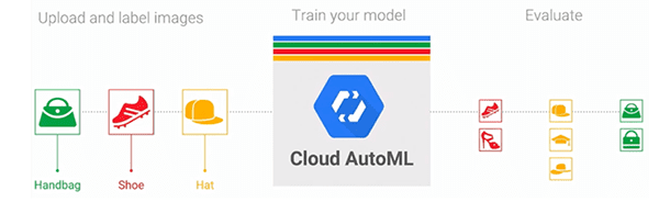
Figure 1: Auto-Keras is an alternative to Google’s AutoML. These software projects can help you train models automatically with little intervention. They are great options for novice deep learning practitioners or to obtain a baseline to beat later on.

在无监督学习(从未标记数据中自动学习模式)之外，面向非专家的自动化机器学习被认为是机器学习的“圣杯”。

想象一下通过以下方式自动创建机器学习模型的能力:

1. 安装库/使用 web 界面
2. 将库/接口指向您的数据
3. 根据数据自动训练模型，而不必调整参数/需要深入了解驱动它的算法

一些公司正试图创造这样的解决方案——一个大的例子是谷歌的 AutoML。

Google AutoML 使机器学习经验非常有限的开发人员和工程师能够在自己的数据集上自动训练神经网络。

在引擎盖下，谷歌的 AutoML 算法是迭代的:

1. 在训练集上训练网络
2. 在测试集上评估网络
3. 修改神经网络架构
4. 调谐超参数
5. 重复这个过程

使用 AutoML 的程序员或工程师不需要定义他们自己的神经网络架构或调整超参数——AutoML 会自动为他们完成这些工作。

神经结构搜索(NAS)使 AutoML 成为可能

Figure 2: Neural Architecture Search (NAS) produced a model summarized by these graphs when searching for the best CNN architecture for CIFAR-10 (source: Figure 4 of Zoph et al.)

谷歌的 AutoML 和 Auto-Keras 都是由一种叫做神经架构搜索(NAS)的算法驱动的。

给定你的输入数据集，一个神经结构搜索算法将自动搜索最佳的结构和相应的参数。

神经架构搜索本质上是用一套自动调优模型的算法来代替深度学习工程师/从业者！

在计算机视觉和图像识别的背景下，神经架构搜索算法将:

1. 接受输入训练数据集
2. 优化并找到称为“单元”的架构构建块——这些单元是自动学习的，可能看起来类似于初始、剩余或挤压/发射微架构
3. 不断训练和搜索“NAS 搜索空间”以获得更优化的单元

如果 AutoML 系统的用户是经验丰富的深度学习实践者，那么他们可以决定:

1. 在训练数据集的一个非常小的子集上运行 NAS
2. 找到一组最佳的架构构建块/单元
3. 获取这些单元，并手动定义在架构搜索期间发现的网络的更深版本
4. 使用他们自己的专业知识和最佳实践对网络进行全面培训

这样的方法是完全自动化的机器学习解决方案和需要专业深度学习实践者的解决方案之间的混合——通常这种方法会比 NAS 自己发现的方法更准确。

我建议阅读 带强化学习的神经架构搜索 (Zoph 和 Le，2016)以及 学习可扩展图像识别的可转移架构 (Zoph 等人，2017)，以了解这些算法如何工作的更多详细信息。

auto-Keras:Google AutoML 的开源替代方案

Figure 3: The Auto-Keras package was developed by the DATA Lab team at Texas A&M University. Auto-Keras is an open source alternative to Google’s AutoML.

由德克萨斯 A & M 大学的数据实验室团队开发的 Auto-Keras 软件包是谷歌 AutoML 的替代产品。

Auto-Keras 还利用神经架构搜索，但应用“网络态射”(在改变架构时保持网络功能)以及贝叶斯优化来指导网络态射，以实现更高效的神经网络搜索。

你可以在金等人的 2018 年出版物中找到 Auto-Keras 框架的完整细节， Auto-Keras:使用网络态射的高效神经架构搜索 。

项目结构

继续从今天博客文章的 【下载】 部分抓取压缩文件。

从那里你应该解压文件并使用你的终端导航到它。

让我们用tree命令来检查今天的项目:

$ tree --dirsfirst
.
├── output
│   ├── 14400.txt
│   ├── 28800.txt
│   ├── 3600.txt
│   ├── 43200.txt
│   ├── 7200.txt
│   └── 86400.txt
└── train_auto_keras.py

1 directory, 7 files

今天我们将回顾一个 Python 脚本:train_auto_keras.py。

由于会有大量输出打印到屏幕上，我选择将我们的分类报告(在 scikit-learn 的classification_report工具的帮助下生成)作为文本文件保存到磁盘上。检查上面的output/文件夹，您可以看到一些已经生成的报告。继续在您的终端(cat output/14400.txt)上打印一个，看看它是什么样子。

安装 Auto-Keras

Figure 4: The Auto-Keras package depends upon Python 3.6, TensorFlow, and Keras.

正如 Auto-Keras GitHub 库声明的，Auto-Keras 处于“预发布”状态——这是而不是正式发布。

其次，Auto-Keras 需要 Python 3.6，并且只有兼容 Python 3.6。

如果你使用的是除了 3.6 之外的任何其他版本的 Python，你将能够使用 Auto-Keras 包而不是。

要检查您的 Python 版本，只需使用以下命令:

$ python --version

如果您有 Python 3.6，您可以使用 pip 安装 Auto-Keras:

$ pip install tensorflow # or tensorflow-gpu
$ pip install keras
$ pip install autokeras

如果您在安装或使用 Auto-Keras 时有任何问题，请确保您在官方的 Auto-Keras GitHub 问题页面上发帖，作者将能够帮助您。

用 Auto-Keras 实现我们的培训脚本

让我们继续使用 Auto-Keras 实现我们的培训脚本。打开train_auto_keras.py文件并插入以下代码:

# import the necessary packages
from sklearn.metrics import classification_report
from keras.datasets import cifar10
import autokeras as ak
import os

def main():
	# initialize the output directory
	OUTPUT_PATH = "output"

首先，我们在第 2-5 行导入必要的包:

• 如前所述，我们将使用 scikit-learn 的classification_report来计算统计数据，并将其保存在输出文件中。
• 我们将使用 CIFAR-10 数据集，它方便地内置在keras.datasets中。
• 接下来是我们最显著的导入，autokeras，为了简化，我将其导入为ak。
• 需要os模块，因为我们将在构建输出文件路径时在各种操作系统上容纳路径分隔符。

让我们在第 7 行为我们的脚本定义main函数。由于 Auto-Keras 和 TensorFlow 处理线程的方式，我们需要将代码包装在一个main函数中。详见本 GitHub 发布线程。

我们的基地OUTPUT_PATH定义在线 9 上。

现在，让我们初始化自动 Keras 的训练时间列表:

	# initialize the list of training times that we'll allow
	# Auto-Keras to train for
	TRAINING_TIMES = [
		60 * 60,		# 1 hour
		60 * 60 * 2,	# 2 hours
		60 * 60 * 4,	# 4 hours
		60 * 60 * 8,	# 8 hours
		60 * 60 * 12,	# 12 hours
		60 * 60 * 24,	# 24 hours
	]

第 13-20 行定义了一组TRAINING_TIMES ，包括[1, 2, 4, 8, 12, 24]小时。今天，我们将使用 Auto-Keras 探索更长的训练时间对准确性的影响。

让我们加载 CIFAR-10 数据集并初始化类名:

	# load the training and testing data, then scale it into the
	# range [0, 1]
	print("[INFO] loading CIFAR-10 data...")
	((trainX, trainY), (testX, testY)) = cifar10.load_data()
	trainX = trainX.astype("float") / 255.0
	testX = testX.astype("float") / 255.0

	# initialize the label names for the CIFAR-10 dataset
	labelNames = ["airplane", "automobile", "bird", "cat", "deer",
		"dog", "frog", "horse", "ship", "truck"]

我们的 CIFAR-10 数据被加载并存储到线 25 上的训练/测试分割中。

随后，我们将把这个数据缩放到范围*【0，1】*(第 26 行和第 27 行)。

我们的类labelNames在行的第 30 行和第 31 行被初始化。这 10 个类包含在 CIFAR-10 中。请注意，顺序在这里很重要。

现在让我们开始循环我们的TRAINING_TIMES，每次都使用 Auto-Keras:

	# loop over the number of seconds to allow the current Auto-Keras
	# model to train for
	for seconds in TRAINING_TIMES:
		# train our Auto-Keras model
		print("[INFO] training model for {} seconds max...".format(
			seconds))
		model = ak.ImageClassifier(verbose=True)
		model.fit(trainX, trainY, time_limit=seconds)
		model.final_fit(trainX, trainY, testX, testY, retrain=True)

		# evaluate the Auto-Keras model
		score = model.evaluate(testX, testY)
		predictions = model.predict(testX)
		report = classification_report(testY, predictions,
			target_names=labelNames)

		# write the report to disk
		p = os.path.sep.join(OUTPUT_PATH, "{}.txt".format(seconds))
		f = open(p, "w")
		f.write(report)
		f.write("\nscore: {}".format(score))
		f.close()

上面的代码块是今天脚本的核心。在第 35 行的上，我们定义了一个循环，其中我们:

• 初始化我们的model ( ak.ImageClassifier)并允许训练开始(第 39 和 40 行)。请注意，我们没有像在之前的教程中一样为特定的 CNN 类实例化一个对象，比如这个。我们也不需要像通常那样调整超参数。Auto-Keras 为我们处理所有这些问题，并提供其调查结果报告。
• 一旦达到时间限制，采用 Auto-Keras 找到的最佳model和参数+重新训练模型(第 41 行)。
• 评估并构建分类report ( 第 44-47 行)。
• 将分类report和精度score写入磁盘，这样我们可以评估更长训练时间的影响(第 50-54 行)。

我们将对每个TRAINING_TIMES重复这个过程。

最后，我们将检查并启动执行的main线程:

# if this is the main thread of execution then start the process (our
# code must be wrapped like this to avoid threading issues with
# TensorFlow)
if __name__ == "__main__":
	main()

这里我们已经检查过，确保这是执行的main线程，然后是main函数。

仅仅 60 行代码之后，我们就完成了使用 CIFAR-10 示例脚本编写 Auto-Keras 的工作。但是我们还没有完成…

用 Auto-kers 训练神经网络

让我们继续使用 Auto-Keras 训练我们的神经网络。

确保使用本教程的 【下载】 部分下载源代码。

从那里，打开一个终端，导航到您下载源代码的位置，并执行以下命令:

$ python train_auto_keras.py
[INFO] training model for 3600 seconds max...   
Preprocessing the images.
Preprocessing finished.

Initializing search.
Initialization finished.

+----------------------------------------------+
|               Training model 0               |
+----------------------------------------------+
Using TensorFlow backend.

No loss decrease after 5 epochs.

Saving model.
+--------------------------------------------------------------------------+
|        Model ID        |          Loss          |      Metric Value      |
+--------------------------------------------------------------------------+
|           0            |   4.816269397735596    |         0.5852         |
+--------------------------------------------------------------------------+

+----------------------------------------------+
|               Training model 1               |
+----------------------------------------------+
Using TensorFlow backend.
Epoch-14, Current Metric - 0.83:  28%|██████▊                 | 110/387 [01:02<02:46,  1.67 batch/s]Time is out.
[INFO] training model for 86400 seconds max...  
Preprocessing the images.
Preprocessing finished.

Initializing search.
Initialization finished.

+----------------------------------------------+
|               Training model 0               |
+----------------------------------------------+
Using TensorFlow backend.

No loss decrease after 5 epochs.
...
+----------------------------------------------+
|              Training model 21               |
+----------------------------------------------+
Using TensorFlow backend.

No loss decrease after 5 epochs.

+--------------------------------------------------------------------------+
|    Father Model ID     |                 Added Operation                 |
+--------------------------------------------------------------------------+
|                        |             to_deeper_model 16 ReLU             |
|           16           |               to_wider_model 16 64              |
+--------------------------------------------------------------------------+

Saving model.
+--------------------------------------------------------------------------+
|        Model ID        |          Loss          |      Metric Value      |
+--------------------------------------------------------------------------+
|           21           |   0.8843476831912994   |   0.9316000000000001   |
+--------------------------------------------------------------------------+

+----------------------------------------------+
|              Training model 22               |
+----------------------------------------------+
Using TensorFlow backend.
Epoch-3, Current Metric - 0.9:  80%|████████████████████▊     | 310/387 [03:50<00:58,  1.31 batch/s]Time is out.

No loss decrease after 30 epochs.

在这里，您可以看到我们的脚本指示 Auto-Keras 执行六组实验。

在 NVIDIA K80 GPU 上，包括时间限制+重新适应模型的时间在内的总训练时间为 3 天多一点。

自动 Keras 结果

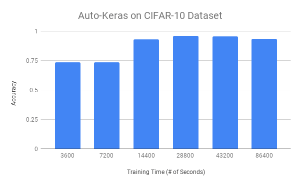
Figure 5: Using Auto-Keras usually is a very time-consuming process. Training with Auto-Keras produces the best models for CIFAR-10 in the 8-12 hour range. Past that, Auto-Keras is not able to optimize further.

在上面的图 5 中，您可以看到使用 Auto-Keras 的训练时间(x-轴)对整体精度(y-轴)的影响。

较低的训练时间，即 1 和 2 小时，导致约 73%的准确率。一旦我们训练了 4 个小时，我们就能达到 93%的准确率。

我们获得的最佳精度在 8-12 范围内，在此范围内我们达到了 95%的精度。

超过 8-12 小时的训练不会增加我们的准确性，这意味着我们已经达到了饱和点，Auto-Keras 不能进一步优化。

Auto-Keras 和 AutoML 值得吗？

Figure 6: Is Auto-Keras (or AutoML) worth it? It is certainly a great step forward in the industry and is especially helpful for those without deep learning domain knowledge. That said, seasoned deep learning experts can craft architectures + train them in significantly less time + achieve equal or greater accuracy.

在无监督学习(从未标记数据中自动学习模式)之外，面向非专家的自动化机器学习被认为是机器学习的“圣杯”。

谷歌的 AutoML 和开源的 Auto-Keras 包都试图将机器学习带给大众，即使没有丰富的技术经验。

虽然 Auto-Keras 在 CIFAR-10 上工作得相当好，但我使用我之前关于深度学习、医学成像和疟疾检测的帖子运行了第二组实验。

在之前的那篇文章中，我使用一个简化的 ResNet 架构获得了 97.1%的准确率，训练时间不到一个小时。

然后，我让 Auto-Keras 在同一个数据集上运行 24 小时——结果只有 96%的准确率，低于我手动定义的架构。

谷歌的 AutoML 和 Auto-Keras 都是巨大的进步；然而，自动化机器学习还远未解决。

自动机器学习(目前)无法击败深度学习方面的专业知识——领域专业知识，特别是你正在处理的数据，对于获得更高精度的模型来说是绝对关键的。

我的建议是投资你自己的知识，不要依赖自动化算法。

要成为一名成功的深度学习实践者和工程师，你需要为工作带来正确的工具。使用 AutoML 和 Auto-Keras，它们是什么，工具，然后继续用额外的知识填充你自己的工具箱。

摘要

在今天的博文中，我们讨论了 Auto-Keras 和 AutoML，这是一组用于执行自动化机器学习和深度学习的工具和库。

Auto-Keras 和 AutoML 的最终目标都是通过使用神经架构搜索(NAS)算法来降低执行机器学习和深度学习的门槛。

NAS 算法，Auto-Keras 和 AutoML 的主干，将自动 :

1. 定义和优化神经网络架构
2. 根据模型调整超参数

主要优势包括:

• 能够在几乎没有专业知识的情况下执行机器学习和深度学习
• 获得高精度模型，该模型能够推广到训练和测试集之外的数据
• 使用 GUI 界面或简单的 API 快速启动和运行
• 不费吹灰之力就有可能达到艺术水平的表演

当然，这是要付出代价的——事实上是两种代价。

首先，谷歌的 AutoML 很贵，大约 20 美元/小时。

为了节省资金，你可以使用 Auto-Keras，这是谷歌 AutoML 的一个开源替代品，但你仍然需要为 GPU 计算时间付费。

用 NAS 算法替换实际的深度学习专家将需要许多小时的计算来搜索最佳参数。

虽然我们实现了 CIFAR-10 的高精度模型(约 96%的精度)，但当我将 Auto-Keras 应用于我之前关于医学深度学习和疟疾预测的帖子时， Auto-Keras 仅实现了 96.1%的精度，比我的 97%的精度低了整整一个百分点(Auto-Keras 要求多 2300%的计算时间！ )

虽然 Auto-Keras 和 AutoML 在自动化机器学习和深度学习方面可能是朝着正确方向迈出的一步，但在这一领域仍有相当多的工作要做。

没有现成算法解决机器学习/深度学习的灵丹妙药。相反，我建议你投资自己成为一名深度学习实践者和工程师。

你今天和明天学到的技能将在未来获得巨大的回报。

我希望你喜欢今天的教程！

要下载这篇文章的源代码(并在未来教程在 PyImageSearch 上发布时得到通知)，只需在下面的表格中输入您的电子邮件地址！*

使用 Keras 和 TensorFlow 进行基于内容的图像检索的自动编码器

原文：https://pyimagesearch.com/2020/03/30/autoencoders-for-content-based-image-retrieval-with-keras-and-tensorflow/

在本教程中，您将学习如何使用卷积自动编码器，通过 Keras 和 TensorFlow 创建一个基于内容的图像检索系统(即图像搜索引擎)。

几周前，我撰写了一系列关于自动编码器的教程:

1. 第一部分: 自动编码器简介
2. 第二部分: 去噪自动编码器
3. 第三部分: 用自动编码器进行异常检测

这些教程大受欢迎；然而，我没有触及的一个话题是基于内容的图像检索(CBIR) ，这实际上只是一个用于图像搜索引擎的花哨的学术词汇。

图像搜索引擎类似于文本搜索引擎，只是没有向搜索引擎提供文本查询，而是提供了图像查询 — 。然后，图像搜索引擎在其数据库中找到所有视觉上相似/相关的图像，并将其返回给您(就像文本搜索引擎返回文章、博客帖子等的链接一样。).

基于深度学习的 CBIR 和图像检索可以被框定为一种形式的无监督学习:

• 当训练自动编码器时，我们不使用任何类别标签
• 然后，自动编码器用于计算我们数据集中每个图像的潜在空间向量表示(即，给定图像的“特征向量”)
• 然后，在搜索时，我们计算潜在空间向量之间的距离——距离更小，更相关/视觉上相似两幅图像是

因此，我们可以将 CBIR 项目分为三个不同的阶段:

1. 阶段#1: 训练自动编码器
2. 阶段#2: 通过使用自动编码器计算图像的潜在空间表示，从数据集中的所有图像中提取特征
3. 阶段#3: 比较潜在空间向量以找到数据集中的所有相关图像

在本教程中，我将向您展示如何实现这些阶段，给您留下一个功能齐全的自动编码器和图像检索系统。

要了解如何使用自动编码器通过 Keras 和 TensorFlow 进行图像检索，请继续阅读！

使用 Keras 和 TensorFlow 进行基于内容的图像检索的自动编码器

在本教程的第一部分，我们将讨论如何自动编码器可以用于图像检索和建立图像搜索引擎。

从那里，我们将实现一个卷积自动编码器，然后在我们的图像数据集上进行训练。

一旦自动编码器被训练，我们将为数据集中的每幅图像计算特征向量。计算给定图像的特征向量只需要图像通过网络向前传递——编码器的输出(即潜在空间表示)将作为我们的特征向量。

所有图像编码后，我们可以通过计算矢量之间的距离来比较矢量。距离较小的图像将比距离较大的图像更相似。

最后，我们将回顾应用我们的自动编码器进行图像检索的结果。

如何将自动编码器用于图像检索和图像搜索引擎？

正如在我的自动编码器简介教程中所讨论的，自动编码器:

1. 接受一组输入数据(即输入)
2. 在内部将输入数据压缩成一个潜在空间表示(即压缩和量化输入的单个向量)
3. 从这个潜在表示(即输出)中重建输入数据

为了用自动编码器建立一个图像检索系统，我们真正关心的是潜在空间表示向量。

一旦自动编码器被训练编码图像，我们就可以:

1. 使用网络的编码器部分来计算我们的数据集中每个图像的潜在空间表示— 该表示用作我们的特征向量，其量化图像的内容
2. 将查询图像的特征向量与数据集中的所有特征向量进行比较(通常使用欧几里德距离或余弦距离)

具有较小距离的特征向量将被认为更相似，而具有较大距离的图像将被认为不太相似。

然后，我们可以根据距离(从最小到最大)对结果进行排序，并最终向最终用户显示图像检索结果。

项目结构

继续从 “下载” 部分获取本教程的文件。从那里，提取。zip，并打开文件夹进行检查:

$ tree --dirsfirst
.
├── output
│   ├── autoencoder.h5
│   ├── index.pickle
│   ├── plot.png
│   └── recon_vis.png
├── pyimagesearch
│   ├── __init__.py
│   └── convautoencoder.py
├── index_images.py
├── search.py
└── train_autoencoder.py

2 directories, 9 files

本教程由三个 Python 驱动程序脚本组成:

• train_autoencoder.py:使用ConvAutoencoder CNN/class 在 MNIST 手写数字数据集上训练一个自动编码器
• index_images.py:使用我们训练过的自动编码器的编码器部分，我们将计算数据集中每个图像的特征向量，并将这些特征添加到可搜索的索引中
• search.py:使用相似性度量查询相似图像的索引

我们的output/目录包含我们训练过的自动编码器和索引。训练还会产生一个训练历史图和可视化图像，可以导出到output/文件夹。

为图像检索实现我们的卷积自动编码器架构

在训练我们的自动编码器之前，我们必须首先实现架构本身。为此，我们将使用 Keras 和 TensorFlow。

我们之前已经在 PyImageSearch 博客上实现过几次卷积自动编码器，所以当我今天在这里报道完整的实现时，你会想要参考我的自动编码器简介教程以获得更多细节。

在pyimagesearch模块中打开convautoencoder.py文件，让我们开始工作:

# import the necessary packages
from tensorflow.keras.layers import BatchNormalization
from tensorflow.keras.layers import Conv2D
from tensorflow.keras.layers import Conv2DTranspose
from tensorflow.keras.layers import LeakyReLU
from tensorflow.keras.layers import Activation
from tensorflow.keras.layers import Flatten
from tensorflow.keras.layers import Dense
from tensorflow.keras.layers import Reshape
from tensorflow.keras.layers import Input
from tensorflow.keras.models import Model
from tensorflow.keras import backend as K
import numpy as np

导入包括来自tf.keras和 NumPy 的选择。接下来我们将继续定义我们的 autoencoder 类:

class ConvAutoencoder:
	@staticmethod
	def build(width, height, depth, filters=(32, 64), latentDim=16):
		# initialize the input shape to be "channels last" along with
		# the channels dimension itself
		# channels dimension itself
		inputShape = (height, width, depth)
		chanDim = -1

		# define the input to the encoder
		inputs = Input(shape=inputShape)
		x = inputs

		# loop over the number of filters
		for f in filters:
			# apply a CONV => RELU => BN operation
			x = Conv2D(f, (3, 3), strides=2, padding="same")(x)
			x = LeakyReLU(alpha=0.2)(x)
			x = BatchNormalization(axis=chanDim)(x)

		# flatten the network and then construct our latent vector
		volumeSize = K.int_shape(x)
		x = Flatten()(x)
		latent = Dense(latentDim, name="encoded")(x)

我们的ConvAutoencoder类包含一个静态方法build，它接受五个参数:(1) width、(2) height、(3) depth、(4) filters和(5) latentDim。

然后为编码器定义了Input，此时我们使用 Keras 的功能 API 循环遍历我们的filters并添加我们的CONV => LeakyReLU => BN层集合(第 21-33 行)。

然后我们拉平网络，构建我们的潜在向量 ( 第 36-38 行)。

潜在空间表示是我们数据的压缩形式— 一旦经过训练，这一层的输出将是我们用于量化和表示输入图像内容的特征向量。

从这里开始，我们将构建网络解码器部分的输入:

		# start building the decoder model which will accept the
		# output of the encoder as its inputs
		x = Dense(np.prod(volumeSize[1:]))(latent)
		x = Reshape((volumeSize[1], volumeSize[2], volumeSize[3]))(x)

		# loop over our number of filters again, but this time in
		# reverse order
		for f in filters[::-1]:
			# apply a CONV_TRANSPOSE => RELU => BN operation
			x = Conv2DTranspose(f, (3, 3), strides=2,
				padding="same")(x)
			x = LeakyReLU(alpha=0.2)(x)
			x = BatchNormalization(axis=chanDim)(x)

		# apply a single CONV_TRANSPOSE layer used to recover the
		# original depth of the image
		x = Conv2DTranspose(depth, (3, 3), padding="same")(x)
		outputs = Activation("sigmoid", name="decoded")(x)

		# construct our autoencoder model
		autoencoder = Model(inputs, outputs, name="autoencoder")

		# return the autoencoder model
		return autoencoder

解码器模型接受编码器的输出作为其输入(行 42 和 43 )。

以相反的顺序循环通过filters，我们构造CONV_TRANSPOSE => LeakyReLU => BN层块(第 47-52 行)。

第 56-63 行恢复图像的原始depth。

最后，我们构造并返回我们的autoencoder模型(第 60-63 行)。

有关我们实现的更多细节，请务必参考我们的【Keras 和 TensorFlow 自动编码器简介教程。

使用 Keras 和 TensorFlow 创建自动编码器训练脚本

随着我们的自动编码器的实现，让我们继续训练脚本(阶段#1 )。

打开train_autoencoder.py脚本，插入以下代码:

# set the matplotlib backend so figures can be saved in the background
import matplotlib
matplotlib.use("Agg")

# import the necessary packages
from pyimagesearch.convautoencoder import ConvAutoencoder
from tensorflow.keras.optimizers import Adam
from tensorflow.keras.datasets import mnist
import matplotlib.pyplot as plt
import numpy as np
import argparse
import cv2

在**2-12 号线，**我们处理我们的进口。我们将使用matplotlib的"Agg"后端，这样我们可以将我们的训练图导出到磁盘。我们需要前一节中的自定义ConvAutoencoder架构类。当我们在 MNIST 基准数据集上训练时，我们将利用Adam优化器。

为了可视化，我们将在visualize_predictions助手函数中使用 OpenCV:

def visualize_predictions(decoded, gt, samples=10):
	# initialize our list of output images
	outputs = None

	# loop over our number of output samples
	for i in range(0, samples):
		# grab the original image and reconstructed image
		original = (gt[i] * 255).astype("uint8")
		recon = (decoded[i] * 255).astype("uint8")

		# stack the original and reconstructed image side-by-side
		output = np.hstack([original, recon])

		# if the outputs array is empty, initialize it as the current
		# side-by-side image display
		if outputs is None:
			outputs = output

		# otherwise, vertically stack the outputs
		else:
			outputs = np.vstack([outputs, output])

	# return the output images
	return outputs

在visualize_predictions助手中，我们将我们的原始地面实况输入图像(gt)与来自自动编码器(decoded)的输出重建图像进行比较，并生成并排比较蒙太奇。

第 16 行初始化我们的输出图像列表。

然后我们循环遍历samples:

• 抓取原始和重建图像(第 21 和 22 行)
• 并排堆叠一对图像*(第 25 行)*
  ** 垂直堆叠线对*(第 29-34 行)**

**最后，我们将可视化图像返回给调用者( Line 37 )。

我们需要一些命令行参数来让我们的脚本从我们的终端/命令行运行:

# construct the argument parse and parse the arguments
ap = argparse.ArgumentParser()
ap.add_argument("-m", "--model", type=str, required=True,
	help="path to output trained autoencoder")
ap.add_argument("-v", "--vis", type=str, default="recon_vis.png",
	help="path to output reconstruction visualization file")
ap.add_argument("-p", "--plot", type=str, default="plot.png",
	help="path to output plot file")
args = vars(ap.parse_args())

这里我们解析三个命令行参数:

• --model:指向我们训练过的输出 autoencoder 的路径——执行这个脚本的结果
• --vis:输出可视化图像的路径。默认情况下，我们将我们的可视化命名为recon_vis.png
• --plot:matplotlib 输出图的路径。如果终端中未提供该参数，则分配默认值plot.png

既然我们的导入、助手函数和命令行参数已经准备好了，我们将准备训练我们的自动编码器:

# initialize the number of epochs to train for, initial learning rate,
# and batch size
EPOCHS = 20
INIT_LR = 1e-3
BS = 32

# load the MNIST dataset
print("[INFO] loading MNIST dataset...")
((trainX, _), (testX, _)) = mnist.load_data()

# add a channel dimension to every image in the dataset, then scale
# the pixel intensities to the range [0, 1]
trainX = np.expand_dims(trainX, axis=-1)
testX = np.expand_dims(testX, axis=-1)
trainX = trainX.astype("float32") / 255.0
testX = testX.astype("float32") / 255.0

# construct our convolutional autoencoder
print("[INFO] building autoencoder...")
autoencoder = ConvAutoencoder.build(28, 28, 1)
opt = Adam(lr=INIT_LR, decay=INIT_LR / EPOCHS)
autoencoder.compile(loss="mse", optimizer=opt)

# train the convolutional autoencoder
H = autoencoder.fit(
	trainX, trainX,
	validation_data=(testX, testX),
	epochs=EPOCHS,
	batch_size=BS)

在行 51-53 中定义了超参数常数，包括训练时期数、学习率和批量大小。

我们的自动编码器(因此我们的 CBIR 系统)将在 MNIST 手写数字数据集上被训练，我们从磁盘的第 57 行加载该数据集。

为了预处理 MNIST 图像，我们向训练/测试集添加通道维度(行 61 和 62 )并将像素强度缩放到范围*【0，1】*(行 63 和 64 )。

随着我们的数据准备就绪，第 68-70 行 compile我们的autoencoder与Adam优化器和均方差loss。

第 73-77 行然后将我们的模型与数据拟合(即训练我们的autoencoder)。

一旦模型被训练好，我们就可以用它来做预测:

# use the convolutional autoencoder to make predictions on the
# testing images, construct the visualization, and then save it
# to disk
print("[INFO] making predictions...")
decoded = autoencoder.predict(testX)
vis = visualize_predictions(decoded, testX)
cv2.imwrite(args["vis"], vis)

# construct a plot that plots and saves the training history
N = np.arange(0, EPOCHS)
plt.style.use("ggplot")
plt.figure()
plt.plot(N, H.history["loss"], label="train_loss")
plt.plot(N, H.history["val_loss"], label="val_loss")
plt.title("Training Loss and Accuracy")
plt.xlabel("Epoch #")
plt.ylabel("Loss/Accuracy")
plt.legend(loc="lower left")
plt.savefig(args["plot"])

# serialize the autoencoder model to disk
print("[INFO] saving autoencoder...")
autoencoder.save(args["model"], save_format="h5")

第 83 行和第 84 行对测试集进行预测，并使用我们的助手函数生成我们的自动编码器可视化。第 85 行使用 OpenCV 将可视化写入磁盘。

最后，我们绘制培训历史(第 88-97 行)并将我们的autoencoder序列化到磁盘(第 101 行)。

在下一部分中，我们将使用培训脚本。

训练自动编码器

我们现在准备训练我们的卷积自动编码器进行图像检索。

确保使用本教程的 【下载】 部分下载源代码，并从那里执行以下命令开始训练过程:

$ python train_autoencoder.py --model output/autoencoder.h5 \
    --vis output/recon_vis.png --plot output/plot.png
[INFO] loading MNIST dataset...
[INFO] building autoencoder...
Train on 60000 samples, validate on 10000 samples
Epoch 1/20
60000/60000 [==============================] - 73s 1ms/sample - loss: 0.0182 - val_loss: 0.0124
Epoch 2/20
60000/60000 [==============================] - 73s 1ms/sample - loss: 0.0101 - val_loss: 0.0092
Epoch 3/20
60000/60000 [==============================] - 73s 1ms/sample - loss: 0.0090 - val_loss: 0.0084
...
Epoch 18/20
60000/60000 [==============================] - 72s 1ms/sample - loss: 0.0065 - val_loss: 0.0067
Epoch 19/20
60000/60000 [==============================] - 73s 1ms/sample - loss: 0.0065 - val_loss: 0.0067
Epoch 20/20
60000/60000 [==============================] - 73s 1ms/sample - loss: 0.0064 - val_loss: 0.0067
[INFO] making predictions...
[INFO] saving autoencoder...

在我的 3Ghz 英特尔至强 W 处理器上，整个培训过程花费了大约 24 分钟。

查看**图 2、**中的曲线，我们可以看到训练过程是稳定的，没有过度拟合的迹象:

Figure 2: Training an autoencoder with Keras and TensorFlow for Content-based Image Retrieval (CBIR).

此外，下面的重构图表明，我们的自动编码器在重构输入数字方面做得非常好。

Figure 3: Visualizing reconstructed data from an autoencoder trained on MNIST using TensorFlow and Keras for image search engine purposes.

我们的自动编码器做得如此之好的事实也意味着我们的潜在空间表示向量在压缩、量化和表示输入图像方面做得很好——当构建图像检索系统时，拥有这样的表示是要求。

如果特征向量不能捕捉和量化图像的内容，那么CBIR 系统将无法返回相关图像。

如果您发现您的自动编码器无法正确重建图像，那么您的自动编码器不太可能在图像检索方面表现良好。

小心训练一个精确的自动编码器——这样做将有助于确保你的图像检索系统返回相似的图像。

使用经过训练的自动编码器实现图像索引器

随着我们的自动编码器成功训练(阶段#1 ，我们可以继续进行图像检索管道的特征提取/索引阶段(阶段#2 )。

这个阶段至少要求我们使用经过训练的自动编码器(特别是“编码器”部分)来接受输入图像，执行前向传递，然后获取网络编码器部分的输出，以生成我们的特征向量的索引。这些特征向量意味着量化每个图像的内容。

可选地，我们也可以使用专门的数据结构，例如 VP-Trees 和随机投影树来提高我们的图像检索系统的查询速度。

打开目录结构中的index_images.py文件，我们将开始:

# import the necessary packages
from tensorflow.keras.models import Model
from tensorflow.keras.models import load_model
from tensorflow.keras.datasets import mnist
import numpy as np
import argparse
import pickle

# construct the argument parse and parse the arguments
ap = argparse.ArgumentParser()
ap.add_argument("-m", "--model", type=str, required=True,
	help="path to trained autoencoder")
ap.add_argument("-i", "--index", type=str, required=True,
	help="path to output features index file")
args = vars(ap.parse_args())

我们从进口开始。我们的tf.keras导入包括(1) Model以便我们可以构建编码器，(2) load_model以便我们可以加载我们在上一步中训练的自动编码器模型，以及(3)我们的mnist数据集。我们的特征向量索引将被序列化为一个 Python pickle文件。

我们有两个必需的命令行参数:

• --model:上一步训练好的自动编码器输入路径
• --index:输出特征索引文件的路径，格式为.pickle

从这里，我们将加载并预处理我们的 MNIST 数字数据:

# load the MNIST dataset
print("[INFO] loading MNIST training split...")
((trainX, _), (testX, _)) = mnist.load_data()

# add a channel dimension to every image in the training split, then
# scale the pixel intensities to the range [0, 1]
trainX = np.expand_dims(trainX, axis=-1)
trainX = trainX.astype("float32") / 255.0

请注意，预处理步骤与我们训练过程的步骤相同。

然后我们将加载我们的自动编码器:

# load our autoencoder from disk
print("[INFO] loading autoencoder model...")
autoencoder = load_model(args["model"])

# create the encoder model which consists of *just* the encoder
# portion of the autoencoder
encoder = Model(inputs=autoencoder.input,
	outputs=autoencoder.get_layer("encoded").output)

# quantify the contents of our input images using the encoder
print("[INFO] encoding images...")
features = encoder.predict(trainX)

第 28 行从磁盘加载我们的autoencoder(在上一步中训练的)。

然后，使用自动编码器的input，我们创建一个Model，同时只访问网络的encoder部分(即潜在空间特征向量)作为output ( 行 32 和 33 )。

然后，我们将 MNIST 数字图像数据通过encoder来计算第 37 行上的特征向量features。

最后，我们构建了特征数据的字典映射:

# construct a dictionary that maps the index of the MNIST training
# image to its corresponding latent-space representation
indexes = list(range(0, trainX.shape[0]))
data = {
    
    "indexes": indexes, "features": features}

# write the data dictionary to disk
print("[INFO] saving index...")
f = open(args["index"], "wb")
f.write(pickle.dumps(data))
f.close()

第 42 行构建了一个由两部分组成的data字典:

• indexes:数据集中每个 MNIST 数字图像的整数索引
• features:数据集中每幅图像对应的特征向量

最后，第 46-48 行以 Python 的pickle格式将data序列化到磁盘。

为图像检索索引我们的图像数据集

我们现在准备使用自动编码器量化我们的图像数据集，特别是使用网络编码器部分的潜在空间输出。

要使用经过训练的 autoencoder 量化我们的图像数据集，请确保使用本教程的 “下载” 部分下载源代码和预训练模型。

从那里，打开一个终端并执行以下命令:

$ python index_images.py --model output/autoencoder.h5 \
	--index output/index.pickle
[INFO] loading MNIST training split...
[INFO] loading autoencoder model...
[INFO] encoding images...
[INFO] saving index...

如果您检查您的output目录的内容，您现在应该看到您的index.pickle文件:

$ ls output/*.pickle
output/index.pickle

使用 Keras 和 TensorFlow 实现图像搜索和检索脚本

我们的最终脚本，我们的图像搜索器，将所有的片段放在一起，并允许我们完成我们的 autoencoder 图像检索项目(阶段#3 )。同样，我们将在这个实现中使用 Keras 和 TensorFlow。

打开search.py脚本，插入以下内容:

# import the necessary packages
from tensorflow.keras.models import Model
from tensorflow.keras.models import load_model
from tensorflow.keras.datasets import mnist
from imutils import build_montages
import numpy as np
import argparse
import pickle
import cv2

如您所见，这个脚本需要与我们的索引器相同的tf.keras导入。此外，我们将使用我的 imutils 包中的build_montages便利脚本来显示我们的 autoencoder CBIR 结果。

让我们定义一个函数来计算两个特征向量之间的相似性:

def euclidean(a, b):
	# compute and return the euclidean distance between two vectors
	return np.linalg.norm(a - b)

这里我们用欧几里德距离来计算两个特征向量a和b之间的相似度。

有多种方法可以计算距离-对于许多 CBIR 应用程序来说，余弦距离是一种很好的替代方法。我还会在 PyImageSearch 大师课程中介绍其他距离算法。

接下来，我们将定义我们的搜索函数:

def perform_search(queryFeatures, index, maxResults=64):
	# initialize our list of results
	results = []

	# loop over our index
	for i in range(0, len(index["features"])):
		# compute the euclidean distance between our query features
		# and the features for the current image in our index, then
		# update our results list with a 2-tuple consisting of the
		# computed distance and the index of the image
		d = euclidean(queryFeatures, index["features"][i])
		results.append((d, i))

	# sort the results and grab the top ones
	results = sorted(results)[:maxResults]

	# return the list of results
	return results

我们的perform_search函数负责比较所有特征向量的相似性，并返回results。

该函数接受查询图像的特征向量queryFeatures和要搜索的所有特征的index。

我们的results将包含顶部的maxResults(在我们的例子中，64是默认的，但我们很快会将其覆盖为225)。

第 17 行初始化我们的列表results，然后第 20-20 行填充它。这里，我们循环遍历index中的所有条目，计算queryFeatures和index中当前特征向量之间的欧几里德距离。

说到距离:

• 距离越小，两幅图像越相似
• 距离越大，越不相似

我们排序并抓取顶部的results，这样通过第 29 行与查询更相似的图像就在列表的最前面。

最后，我们return将搜索结果传递给调用函数(第 32 行)。

定义了距离度量和搜索工具后，我们现在准备好解析命令行参数:

# construct the argument parse and parse the arguments
ap = argparse.ArgumentParser()
ap.add_argument("-m", "--model", type=str, required=True,
	help="path to trained autoencoder")
ap.add_argument("-i", "--index", type=str, required=True,
	help="path to features index file")
ap.add_argument("-s", "--sample", type=int, default=10,
	help="# of testing queries to perform")
args = vars(ap.parse_args())

我们的脚本接受三个命令行参数:

• --model:从*“训练自动编码器”*部分到被训练自动编码器的路径
• --index:我们要搜索的特征索引(即来自*“为图像检索而索引我们的图像数据集”部分的序列化索引)*
• --sample:要执行的测试查询的数量，默认值为10

现在，让我们加载并预处理我们的数字数据:

# load the MNIST dataset
print("[INFO] loading MNIST dataset...")
((trainX, _), (testX, _)) = mnist.load_data()

# add a channel dimension to every image in the dataset, then scale
# the pixel intensities to the range [0, 1]
trainX = np.expand_dims(trainX, axis=-1)
testX = np.expand_dims(testX, axis=-1)
trainX = trainX.astype("float32") / 255.0
testX = testX.astype("float32") / 255.0

然后我们将加载我们的自动编码器和索引:

# load the autoencoder model and index from disk
print("[INFO] loading autoencoder and index...")
autoencoder = load_model(args["model"])
index = pickle.loads(open(args["index"], "rb").read())

# create the encoder model which consists of *just* the encoder
# portion of the autoencoder
encoder = Model(inputs=autoencoder.input,
	outputs=autoencoder.get_layer("encoded").output)

# quantify the contents of our input testing images using the encoder
print("[INFO] encoding testing images...")
features = encoder.predict(testX)

这里，线 57 从磁盘加载我们训练好的autoencoder，而线 58 从磁盘加载我们腌制好的index。

然后我们构建一个Model，它将接受我们的图像作为一个input和我们的encoder层的output(即特征向量)作为我们模型的输出(第 62 和 63 行)。

给定我们的encoder , 行 67 通过网络向前传递我们的测试图像集，生成一个features列表来量化它们。

我们现在将随机抽取一些图像样本，将它们标记为查询:

# randomly sample a set of testing query image indexes
queryIdxs = list(range(0, testX.shape[0]))
queryIdxs = np.random.choice(queryIdxs, size=args["sample"],
	replace=False)

# loop over the testing indexes
for i in queryIdxs:
	# take the features for the current image, find all similar
	# images in our dataset, and then initialize our list of result
	# images
	queryFeatures = features[i]
	results = perform_search(queryFeatures, index, maxResults=225)
	images = []

	# loop over the results
	for (d, j) in results:
		# grab the result image, convert it back to the range
		# [0, 255], and then update the images list
		image = (trainX[j] * 255).astype("uint8")
		image = np.dstack([image] * 3)
		images.append(image)

	# display the query image
	query = (testX[i] * 255).astype("uint8")
	cv2.imshow("Query", query)

	# build a montage from the results and display it
	montage = build_montages(images, (28, 28), (15, 15))[0]
	cv2.imshow("Results", montage)
	cv2.waitKey(0)

第 70-72 行采样一组测试图像索引，将它们标记为我们的搜索引擎查询。

然后我们从第 75 行的开始循环查询。在内部，我们:

• 抓住queryFeatures，执行搜索(79 行和 80 行)
• 初始化一个列表来保存我们的结果images ( 第 81 行)
• 对结果进行循环，将图像缩放回范围*【0，255】*，从灰度图像创建 RGB 表示用于显示，然后将其添加到我们的images结果中(第 84-89 行)
• 在自己的 OpenCV 窗口中显示查询图像(第 92 行和第 93 行)
• 显示搜索引擎结果中的montage(第 96 行和第 97 行)
• 当用户按下一个键时，我们用一个不同的查询图像重复这个过程(行 98)；您应该在检查结果时继续按键，直到搜索完所有的查询样本

回顾一下我们的搜索脚本，首先我们加载了自动编码器和索引。

然后，我们抓住自动编码器的编码器部分，用它来量化我们的图像(即，创建特征向量)。

从那里，我们创建了一个随机查询图像的样本来测试我们的基于欧氏距离计算的搜索方法。较小的距离表示相似的图像——相似的图像将首先显示，因为我们的results是sorted ( 第 29 行)。

我们搜索了每个查询的索引，在每个剪辑中最多只显示了maxResults。

在下一节中，我们将有机会直观地验证我们基于 autoencoder 的搜索引擎是如何工作的。

使用自动编码器、Keras 和 TensorFlow 的图像检索结果

我们现在可以看到我们的 autoencoder 图像检索系统的运行了！

首先确保你有:

1. 使用本教程的 【下载】 部分下载源代码
2. 执行train_autoencoder.py文件来训练卷积自动编码器
3. 运行index_images.py来量化我们数据集中的每幅图像

从那里，您可以执行search.py脚本来执行搜索:

$ python search.py --model output/autoencoder.h5 \
	--index output/index.pickle
[INFO] loading MNIST dataset...
[INFO] loading autoencoder and index...
[INFO] encoding testing images...

下面的例子提供了一个包含数字9 ( 顶部)的查询图像，以及来自我们的 autoencoder 图像检索系统*(底部)*的搜索结果:

Figure 4: Top: MNIST query image. Bottom: Autoencoder-based image search engine results. We learn how to use Keras, TensorFlow, and OpenCV to build a Content-based Image Retrieval (CBIR) system.

在这里，您可以看到我们的系统返回的搜索结果也包含 9。

现在让我们使用一个2作为我们的查询图像:

Figure 5: Content-based Image Retrieval (CBIR) is used with an autoencoder to find images of handwritten 2s in our dataset.

果然，我们的 CBIR 系统返回包含二的数字，这意味着潜在空间表示已经正确量化了2的样子。

下面是一个使用4作为查询图像的例子:

Figure 6: Content-based Image Retrieval (CBIR) is used with an autoencoder to find images of handwritten 4s in our dataset.

同样，我们的 autoencoder 图像检索系统返回所有四个作为搜索结果。

让我们看最后一个例子，这次使用一个0作为查询图像:

Figure 7: No image search engine is perfect. Here, there are mistakes in our results from searching MNIST for handwritten 0s using an autoencoder-based image search engine built with TensorFlow, Keras, and OpenCV.

这个结果更有趣—注意截图中突出显示的两个结果。

第一个高亮显示的结果可能是一个5，但是五的尾部似乎连接到中间部分，创建了一个数字，看起来像是一个0和一个8之间的交叉。

然后，我们在搜索结果的底部看到我认为是一个8(也用红色突出显示)。同样，我们可以理解我们的图像检索系统是如何将8视为与0在视觉上相似的。

提高 autoencoder 图像检索准确性和速度的技巧

在本教程中，我们在 MNIST 数据集上执行图像检索，以演示如何使用自动编码器来构建图像搜索引擎。

但是，您很可能希望使用自己的影像数据集，而不是 MNIST 数据集。

换入您自己的数据集就像用您自己的数据集加载器替换 MNIST 数据集加载器辅助函数一样简单-然后您可以在您的数据集上训练自动编码器。

然而，确保你的自动编码器足够精确。

如果您的自动编码器无法合理地重建您的输入数据，则:

1. 自动编码器无法捕获数据集中的模式
2. 潜在空间向量不会正确量化你的图像
3. 没有适当的量化，您的图像检索系统将返回不相关的结果

因此，几乎您的 CBIR 系统的整体精度取决于您的自动编码器——请花时间确保它经过适当的培训。

一旦你的自动编码器运行良好，你就可以继续优化搜索过程的速度。

其次，您还应该考虑 CBIR 系统的可扩展性。

我们在这里的实现是一个线性搜索的例子，复杂度为 O(N) ，这意味着它不能很好地扩展。

为了提高检索系统的速度，您应该使用近似最近邻算法和专门的数据结构，如 VP 树、随机投影树等。，可以将计算复杂度降低到 O(log N)。

要了解更多关于这些技术的内容，请参考我的文章用 VP-Trees 和 OpenCV 构建一个图像哈希搜索引擎。

摘要

在本教程中，您学习了如何使用 TensorFlow 和 Keras 将卷积自动编码器用于图像检索。

为了创建我们的图像检索系统，我们:

1. 在我们的图像数据集上训练卷积自动编码器
2. 使用经过训练的自动编码器来计算我们的数据集中每个图像的潜在空间表示——该表示作为我们的特征向量来量化图像的内容
3. 使用距离函数将查询图像的特征向量与数据集中的所有特征向量进行比较(在这种情况下，使用欧几里德距离，但余弦距离也适用)。向量之间的距离越小，我们的图像就越相似。

然后，我们根据计算出的距离对结果进行排序，并向用户显示结果。

自动编码器对于 CBIR 应用来说非常有用— 缺点是它们需要大量的训练数据，这些数据你可能有也可能没有。

更高级的深度学习图像检索系统依赖于连体网络和三重损失来嵌入图像的向量，以便更相似的图像在欧几里得空间中靠得更近，而不太相似的图像离得更远——我将在未来的某个日期讨论这些类型的网络架构和技术。

要下载这篇文章的源代码(包括预先训练的 autoencoder)，只需在下面的表格中输入您的电子邮件地址！**