【KAN】KAN神经网络学习训练营(15)——API 3：样条

企业开发 2025-04-08 12:31:53 阅读次数: 0

一、引言

KAN神经网络（Kolmogorov–Arnold Networks）是一种基于Kolmogorov-Arnold表示定理的新型神经网络架构。该定理指出，任何多元连续函数都可以表示为有限个单变量函数的组合。与传统多层感知机（MLP）不同，KAN通过可学习的激活函数和结构化网络设计，在函数逼近效率和可解释性上展现出潜力。

二、技术与原理简介

1.Kolmogorov-Arnold 表示定理

Kolmogorov-Arnold 表示定理指出，如果是有界域上的多元连续函数，那么它可以写为单个变量的连续函数的有限组合，以及加法的二进制运算。更具体地说，对于光滑 $ff:[0,1]^{^{n}}\rightarrow \mathbb{R}$

$f \left( x \right)=f \left( x_{1}, \cdots,x_{n} \right)= \sum_{q=1}^{2n+1} \Phi_{q} \left( \sum_{p=1}^{n} \phi_{q,p} \left( x_{p} \right) \right)$

其中和。从某种意义上说，他们表明唯一真正的多元函数是加法，因为所有其他函数都可以使用单变量函数和 sum 来编写。然而，这个 2 层宽度 - Kolmogorov-Arnold 表示可能不是平滑的由于其表达能力有限。我们通过以下方式增强它的表达能力将其推广到任意深度和宽度。 $\boldsymbol{\phi_{q,p}:[0,1]\to\mathbb{R}}$ ， $\boldsymbol{\Phi_{q}:\mathbb{R}\to\mathbb{R}(2n+1)}$

2.Kolmogorov-Arnold 网络（KAN）

Kolmogorov-Arnold 表示可以写成矩阵形式

$f(x)=\mathbf{\Phi_{out}}\mathsf{o}\mathbf{\Phi_{in}}\mathsf{o}{}x$

其中

$\mathbf{\Phi}_{\mathrm{in}}=\begin{pmatrix}\phi_{1,1}(\cdot)&\cdots&\phi_{1,n }(\cdot)\\ \vdots&&\vdots\\ \phi_{2n+1,1}(\cdot)&\cdots&\phi_{2n+1,n}(\cdot)\end{pmatrix}$

$\quad\mathbf{ \Phi}_{\mathrm{out}}=\left(\Phi_{1}(\cdot)\quad\cdots\quad\Phi_{2n+1}(\cdot)\right)$

我们注意到和都是以下函数矩阵（包含输入和输出）的特例，我们称之为 Kolmogorov-Arnold 层： $\mathbf{\Phi_{in}} \mathbf{\Phi_{out}} \mathbf{\Phi_{n_{in}n_{out}}}$

其中 $\boldsymbol{n_{\text{in}}=n,n_{\text{out}}=2n+1\Phi_{\text{out}}n_{\text{in}}=2n+1,n_{\text{out}}=1}$ 。

定义层后，我们可以构造一个 Kolmogorov-Arnold 网络只需堆叠层！假设我们有层，层的形状为。那么整个网络是 $Ll^{th} \Phi_{l} \left( n_{l+1},n_{l} \right)$

$\mathbf{KAN(x)}=\mathbf{\Phi_{L-1}}\circ\cdots\circ\mathbf{\Phi_{1}}\circ \mathbf{\Phi_{0}}\circ\mathbf{x}$

相反，多层感知器由线性层和非线错： $\mathbf{W}_{l^{\sigma}}$

$\text{MLP}(\mathbf{x})=\mathbf{W}_{\textit{L-1}}\circ\sigma\circ\cdots\circ \mathbf{W}_{1}\circ\sigma\circ\mathbf{W}_{0}\circ\mathbf{x}$

KAN 可以很容易地可视化。（1） KAN 只是 KAN 层的堆栈。（2）每个 KAN 层都可以可视化为一个全连接层，每个边缘上都有一个1D 函数。

三、代码详解

KANs（科洛莫哥洛夫-阿诺德网络）的一个重要特点是将样条嵌入到神经网络中。然而，样条仅在已知的有界区域内有效于函数近似，而神经网络中的激活范围可能在训练过程中发生变化。因此，我们必须根据这一情况恰当地更新网格。首先，让我们了解一下我们是如何参数化样条的。

from kan.spline import B_batch
import torch
import matplotlib.pyplot as plt
import numpy as np

# consider a 1D example.
# Suppose we have grid in [-1,1] with G intervals, spline order k
G = 5
k = 3
grid = torch.linspace(-1,1,steps=G+1)[None,:]

# and we have sample range in [-1,1]
x = torch.linspace(-1,1,steps=1001)[None,:]

basis = B_batch(x, grid, k=k)

for i in range(G+k):
    plt.plot(x[0].detach().numpy(), basis[0,i,:].detach().numpy())
    
plt.legend(['B_{}(x)'.format(i) for i in np.arange(G+k)])
plt.xlabel('x')
plt.ylabel('B_i(x)')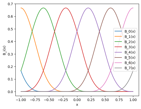

from kan import KAN

model = KAN(width=[1,1], grid=G, k=k)
# obtain coefficients c_i
model.act_fun[0].coef
assert(model.act_fun[0].coef[0].shape[0] == G+k)

# the model forward
model_output = model(x[0][:,None])

# spline output
spline_output = torch.einsum('i,ij->j',model.act_fun[0].coef[0], basis[0])[:,None]

torch.mean((model_output - spline_output)**2)

tensor(0.1382, grad_fn=<MeanBackward0>)

# residual output
residual_output = torch.nn.SiLU()(x[0][:,None])
scale_base = model.act_fun[0].scale_base
scale_sp = model.act_fun[0].scale_sp
torch.mean((model_output - (scale_base * residual_output + scale_sp * spline_output))**2)

tensor(0., grad_fn=<MeanBackward0>)

model = KAN(width=[1,1], grid=G, k=k)
print(model.act_fun[0].grid) # by default, the grid is in [-1,1]
x = torch.linspace(-10,10,steps = 1001)[:,None]
model.update_grid_from_samples(x)
print(model.act_fun[0].grid) # now the grid becomes in [-10,10]. We add a 0.01 margin in case x have zero variance

Parameter containing:
tensor([[-1.0000, -0.6000, -0.2000, 0.2000, 0.6000, 1.0000]])
Parameter containing:
tensor([[-10.0100, -6.0060, -2.0020, 2.0020, 6.0060, 10.0100]])

model = KAN(width=[1,1], grid=G, k=k)
print(model.act_fun[0].grid) # by default, the grid is in [-1,1]
x = torch.linspace(-0.5,0.5,steps = 1001)[:,None]
model.update_grid_from_samples(x)
print(model.act_fun[0].grid) # now the grid becomes in [-10,10]. We add a 0.01 margin in case x have zero variance

Parameter containing:
tensor([[-1.0000, -0.6000, -0.2000, 0.2000, 0.6000, 1.0000]])
Parameter containing:
tensor([[-0.5100, -0.3060, -0.1020, 0.1020, 0.3060, 0.5100]])

# uniform grid
model = KAN(width=[1,1], grid=G, k=k)
print(model.act_fun[0].grid) # by default, the grid is in [-1,1]
x = torch.normal(0,1,size=(1000,1))
model.update_grid_from_samples(x)
print(model.act_fun[0].grid) # now the grid becomes in [-10,10]. We add a 0.01 margin in case x have zero variance

Parameter containing:
tensor([[-1.0000, -0.6000, -0.2000, 0.2000, 0.6000, 1.0000]])
Parameter containing:
tensor([[-3.4896, -2.1218, -0.7541, 0.6137, 1.9815, 3.3493]])

# adaptive grid based on sample distribution
model = KAN(width=[1,1], grid=G, k=k, grid_eps = 0.)
print(model.act_fun[0].grid) # by default, the grid is in [-1,1]
x = torch.normal(0,1,size=(1000,1))
model.update_grid_from_samples(x)
print(model.act_fun[0].grid) # now the grid becomes in [-10,10]. We add a 0.01 margin in case x have zero variance

Parameter containing:
tensor([[-1.0000, -0.6000, -0.2000, 0.2000, 0.6000, 1.0000]])
Parameter containing:
tensor([[-3.4796, -0.8529, -0.2272, 0.2667, 0.8940, 3.3393]])

四、总结与思考

KAN神经网络通过融合数学定理与深度学习，为科学计算和可解释AI提供了新思路。尽管在高维应用中仍需突破，但其在低维复杂函数建模上的潜力值得关注。未来可能通过改进计算效率、扩展理论边界，成为MLP的重要补充。

1. KAN网络架构

关键设计：可学习的激活函数：每个网络连接的“权重”被替换为单变量函数（如样条、多项式），而非固定激活函数（如ReLU）。分层结构：输入层和隐藏层之间、隐藏层与输出层之间均通过单变量函数连接，形成多层叠加。参数效率：由于理论保证，KAN可能用更少的参数达到与MLP相当或更好的逼近效果。
示例结构：输入层 → 隐藏层：每个输入节点通过单变量函数 $\phi_{q,i} \left( x_{i} \right)$ 连接到隐藏节点。隐藏层 → 输出层：隐藏节点通过另一组单变量函数 $\psi_{q}$ 组合得到输出。