卷积神经网络学习（一）——基本卷积神经网络搭建

#!/usr/bin/env python
# -*- coding:utf-8 -*-

import tensorflow as tf
from tensorflow.examples.tutorials.mnist import input_data
# number 1 to 10 data
mnist = input_data.read_data_sets('MNIST_data',one_hot=True)

# 输出结果依然是准确度
def compute_accuracy(v_xs, v_ys):
    global prediction
    y_pre = sess.run(prediction, feed_dict={xs: v_xs, keep_prob: 1})
    correct_prediction = tf.equal(tf.argmax(y_pre,1), tf.argmax(v_ys,1))
    accuracy = tf.reduce_mean(tf.cast(correct_prediction, tf.float32))
    result = sess.run(accuracy, feed_dict={xs: v_xs, ys: v_ys, keep_prob: 1})
    return result

# 定义Weight变量，输入shape，返回变量的参数。其中我们使用tf.truncted_normal产生随机变量来进行初始化:
def weight_variable(shape):
    initial = tf.truncated_normal(shape,stddev=0.1)
    return tf.Variable(initial)

# 定义biase变量，输入shape ,返回变量的一些参数。其中我们使用tf.constant常量函数来进行初始化:
def bias_variable(shape):
    initial = tf.constant(0.1,shape=shape)
    return tf.Variable(initial)

# 定义卷积，tf.nn.conv2d函数是tensoflow里面的二维的卷积函数，x是图片的所有参数，W是此卷积层的权重，然后定义步长
# strides=[1,1,1,1]值，strides[0]和strides[3]的两个1是默认值，中间两个1代表padding时在x方向运动一步，y方向运动一步，padding采用的方式是SAME。
def conv2d(x,W):
    # stride [1,x_movement,y_movement,1]
    return tf.nn.conv2d(x,W,strides=[1,1,1,1],padding='SAME')
    # x为图片的所有信息  strides 步长 水平数值方向跨度都为1

# 为了得到更多的图片信息，padding时选择的是一次一步，也就是strides[1]=strides[2]=1，这样得到的图片尺寸没有变化
# 而我们希望压缩一下图片也就是参数能少一些从而减小系统的复杂度，因此我们采用pooling来稀疏化参数，也就是卷积神经网络中所的下采样层。
# pooling 有两种，一种是最大值池化，一种是平均值池化，本例采用的是最大值池化tf.max_pool()。
# 池化的核函数大小为2x2，因此ksize=[1,2,2,1]，步长为2，因此strides=[1,2,2,1]:
def max_pool_2x2(x):
    return tf.nn.max_pool(x,ksize=[1,2,2,1],strides=[1,2,2,1],padding='SAME')

# define placeholder for inputs to network
xs = tf.placeholder(tf.float32, [None, 784])/255.   # 28x28
ys = tf.placeholder(tf.float32, [None, 10])
# 定义了dropout的placeholder，它是解决过拟合的有效手段
keep_prob = tf.placeholder(tf.float32)
# 先处理xs的信息（传入图片的信息），把xs的形状变成[-1,28,28,1]，-1代表先不考虑输入的图片例子多少这个维度，后面的1是channel的数量，
# 因为我们输入的图片是黑白的，因此channel是1，例如如果是RGB图像，那么channel就是3。
x_image = tf.reshape(xs, [-1, 28, 28, 1])
# print(x_image.shape)  # [n_samples, 28,28,1]

## conv1 layer ##
# 先定义本层的Weight,本层我们的卷积核patch的大小是5x5，因为黑白图片channel是1所以输入是1，输出是32个featuremap
W_conv1 = weight_variable([5, 5, 1, 32]) # patch 5x5, in size 1, out size 32
# 定义bias，它的大小是32个长度，因此我们传入它的shape为[32]
b_conv1 = bias_variable([32])
# 搭建CNN的第一个卷积层，（输入*weight+bias），同时嵌套一个relu的非线性处理，也就是激活函数。
h_conv1 = tf.nn.relu(conv2d(x_image, W_conv1) + b_conv1) # 由于采用SAME的padding方式，输出图片的大小没有变化，只是厚度变厚了。output size 28x28x32
h_pool1 = max_pool_2x2(h_conv1) # 最后进行pooling处理，output size 14x14x32

## conv2 layer ##
# 定义CNN的第二个卷积层
W_conv2 = weight_variable([5, 5, 32, 64]) # patch 5x5, in size 32, out size 64(假设)
b_conv2 = bias_variable([64])
h_conv2 = tf.nn.relu(conv2d(h_pool1, W_conv2) + b_conv2) # 输入layer1所输出的结果。output size 14x14x64
h_pool2 = max_pool_2x2(h_conv2)                                                 # output size 7x7x64

## fc1 layer ##
# 接下来定义 fully connected layer
W_fc1 = weight_variable([7*7*64, 1024]) # 输入的shape是h_pool2展平了的输出大小: 7x7x64，输出1024
b_fc1 = bias_variable([1024])
# 进入全连接层时, 我们通过tf.reshape()将h_pool2的输出值从一个三维的变为一维的数据, -1表示先不考虑输入图片例子维度, 将上一个输出结果展平.
# 形状变换： [n_samples, 7, 7, 64] ->> [n_samples, 7*7*64]
h_pool2_flat = tf.reshape(h_pool2, [-1, 7*7*64])
h_fc1 = tf.nn.relu(tf.matmul(h_pool2_flat, W_fc1) + b_fc1) # 矩阵相乘
h_fc1_drop = tf.nn.dropout(h_fc1, keep_prob) # 考虑overfitting加入一个dropout处理

## fc2 layer ##
W_fc2 = weight_variable([1024, 10]) # 输入1024，输出10个。[0-9]十个类
b_fc2 = bias_variable([10])
# 用softmax分类器（多分类，输出是各个类的概率）,对我们的输出进行分类
prediction = tf.nn.softmax(tf.matmul(h_fc1_drop, W_fc2) + b_fc2)


# the error between prediction and real data
# 利用交叉熵损失函数来定义我们的cost function
cross_entropy = tf.reduce_mean(-tf.reduce_sum(ys * tf.log(prediction),
                                              reduction_indices=[1]))       # loss
# 用tf.train.AdamOptimizer()作为我们的优化器进行优化，使我们的cross_entropy最小
train_step = tf.train.AdamOptimizer(1e-4).minimize(cross_entropy) # learning rate = 0.0001

sess = tf.Session()
init = tf.global_variables_initializer()
sess.run(init)

# sess.run()时记得要用feed_dict给定义的placeholder喂数据.
for i in range(1000):
    batch_xs, batch_ys = mnist.train.next_batch(100)
    sess.run(train_step, feed_dict={xs: batch_xs, ys: batch_ys, keep_prob: 0.5})
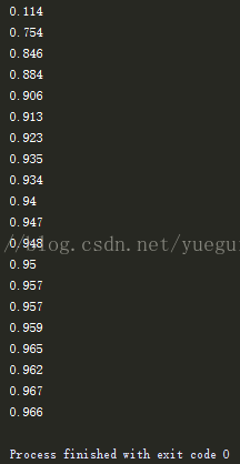
    if i % 50 == 0:
        print(compute_accuracy(
            mnist.test.images[:1000], mnist.test.labels[:1000]))

运行结果：