[六]机器学习之EM算法

6.1 实验概要

通过EM算法解决部分观测数据的参数估计问题，使用sklearn提供的EM模块和高斯混合模型数据集，实验EM算法的实际效果

6.2 实验输入描述

本次实验使用仿真数据集，该数据集有300条数据构成，每个样本为3维。假定该数据由两个高斯分布混合得到。

6.3 实验步骤

（1）手动实现

# !/usr/bin/python
# -*- coding:utf-8 -*-

import numpy as np
from scipy.stats import multivariate_normal
from sklearn.mixture import GaussianMixture
from mpl_toolkits.mplot3d import Axes3D
import matplotlib as mpl
import matplotlib.pyplot as plt
from sklearn.metrics.pairwise import pairwise_distances_argmin


mpl.rcParams['font.sans-serif'] = ['SimHei']
mpl.rcParams['axes.unicode_minus'] = False


if __name__ == '__main__':
    style = 'myself'

    np.random.seed(0)
    mu1_fact = (0, 0, 0)
    cov1_fact = np.diag((1, 2, 3))
    data1 = np.random.multivariate_normal(mu1_fact, cov1_fact*0.1, 400)
    mu2_fact = (2, 2, 1)
    cov2_fact = np.array(((6, 1, 3), (1, 5, 1), (3, 1, 4)))
    data2 = np.random.multivariate_normal(mu2_fact, cov2_fact*0.1, 100)
    data = np.vstack((data1, data2))
    y = np.array([True] * 400 + [False] * 100)

    if style == 'sklearn':
        g = GaussianMixture(n_components=2, covariance_type='full', tol=1e-6, max_iter=1000)
        g.fit(data)
        print u'类别概率:\t', g.weights_[0]
        print u'均值:\n', g.means_, '\n'
        print u'方差:\n', g.covariances_, '\n'
        mu1, mu2 = g.means_
        sigma1, sigma2 = g.covariances_
    else:
        num_iter = 100
        n, d = data.shape
        # 随机指定
        # mu1 = np.random.standard_normal(d)
        # print mu1
        # mu2 = np.random.standard_normal(d)
        # print mu2
        mu1 = data.min(axis=0)
        mu2 = data.max(axis=0)
        print mu1, mu2
        sigma1 = np.identity(d)
        sigma2 = np.identity(d)
        pi = 0.5
        # EM
        for i in range(num_iter):
            # E Step
            norm1 = multivariate_normal(mu1, sigma1)
            norm2 = multivariate_normal(mu2, sigma2)
            tau1 = pi * norm1.pdf(data)
            tau2 = (1 - pi) * norm2.pdf(data)
            gamma = tau1 / (tau1 + tau2)

            # M Step
            mu1 = np.dot(gamma, data) / np.sum(gamma)
            mu2 = np.dot((1 - gamma), data) / np.sum((1 - gamma))
            sigma1 = np.dot(gamma * (data - mu1).T, data - mu1) / np.sum(gamma)
            sigma2 = np.dot((1 - gamma) * (data - mu2).T, data - mu2) / np.sum(1 - gamma)
            pi = np.sum(gamma) / n
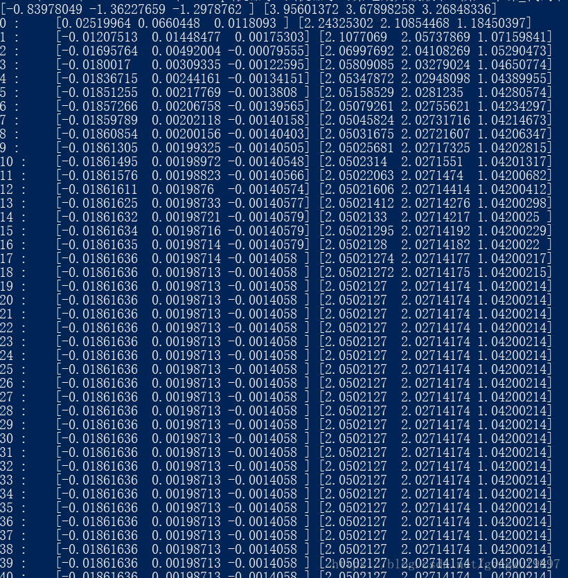
            print i, ":\t", mu1, mu2
        print u'类别概率:\t', pi
        print u'均值:\t', mu1, mu2
        print u'方差:\n', sigma1, '\n\n', sigma2, '\n'

    # 预测分类
    norm1 = multivariate_normal(mu1, sigma1)
    norm2 = multivariate_normal(mu2, sigma2)
    tau1 = norm1.pdf(data)
    tau2 = norm2.pdf(data)

    fig = plt.figure(figsize=(10, 5), facecolor='w')
    ax = fig.add_subplot(121, projection='3d')
    ax.scatter(data[:, 0], data[:, 1], data[:, 2], c='b', s=30, marker='o', edgecolors='k', depthshade=True)
    ax.set_xlabel('X')
    ax.set_ylabel('Y')
    ax.set_zlabel('Z')
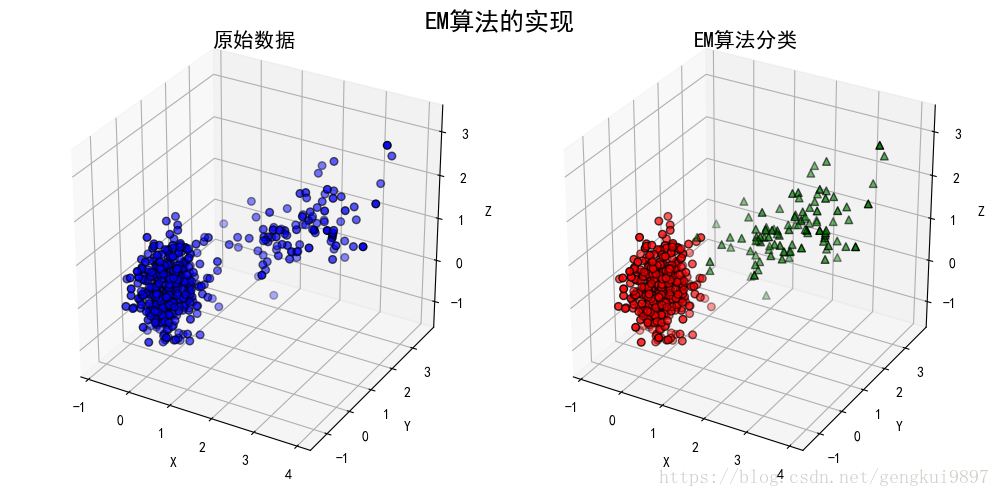
    ax.set_title(u'原始数据', fontsize=15)
    ax = fig.add_subplot(122, projection='3d')
    order = pairwise_distances_argmin([mu1_fact, mu2_fact], [mu1, mu2], metric='euclidean')
    print order
    if order[0] == 0:
        c1 = tau1 > tau2
    else:
        c1 = tau1 < tau2
    c2 = ~c1
    acc = np.mean(y == c1)
    print u'准确率：%.2f%%' % (100*acc)
    ax.scatter(data[c1, 0], data[c1, 1], data[c1, 2], c='r', s=30, marker='o', edgecolors='k', depthshade=True)
    ax.scatter(data[c2, 0], data[c2, 1], data[c2, 2], c='g', s=30, marker='^', edgecolors='k', depthshade=True)
    ax.set_xlabel('X')
    ax.set_ylabel('Y')
    ax.set_zlabel('Z')
    ax.set_title(u'EM算法分类', fontsize=15)
    plt.suptitle(u'EM算法的实现', fontsize=18)
    plt.subplots_adjust(top=0.90)
    plt.tight_layout()
    plt.show()

（2）sklearn库实现

# !/usr/bin/python
# -*- coding:utf-8 -*-

import numpy as np
from scipy.stats import multivariate_normal
from sklearn.mixture import GaussianMixture
from mpl_toolkits.mplot3d import Axes3D
import matplotlib as mpl
import matplotlib.pyplot as plt
from sklearn.metrics.pairwise import pairwise_distances_argmin


mpl.rcParams['font.sans-serif'] = ['SimHei']
mpl.rcParams['axes.unicode_minus'] = False


if __name__ == '__main__':
    style = 'sklearn'

    np.random.seed(0)
    mu1_fact = (0, 0, 0)
    cov1_fact = np.diag((1, 2, 3))
    data1 = np.random.multivariate_normal(mu1_fact, cov1_fact*0.1, 400)
    mu2_fact = (2, 2, 1)
    cov2_fact = np.array(((6, 1, 3), (1, 5, 1), (3, 1, 4)))
    data2 = np.random.multivariate_normal(mu2_fact, cov2_fact*0.1, 100)
    data = np.vstack((data1, data2))
    y = np.array([True] * 400 + [False] * 100)

    if style == 'sklearn':
        g = GaussianMixture(n_components=2, covariance_type='full', tol=1e-6, max_iter=1000)
        g.fit(data)
        print u'类别概率:\t', g.weights_[0]
        print u'均值:\n', g.means_, '\n'
        print u'方差:\n', g.covariances_, '\n'
        mu1, mu2 = g.means_
        sigma1, sigma2 = g.covariances_
    else:
        num_iter = 100
        n, d = data.shape
        # 随机指定
        # mu1 = np.random.standard_normal(d)
        # print mu1
        # mu2 = np.random.standard_normal(d)
        # print mu2
        mu1 = data.min(axis=0)
        mu2 = data.max(axis=0)
        print mu1, mu2
        sigma1 = np.identity(d)
        sigma2 = np.identity(d)
        pi = 0.5
        # EM
        for i in range(num_iter):
            # E Step
            norm1 = multivariate_normal(mu1, sigma1)
            norm2 = multivariate_normal(mu2, sigma2)
            tau1 = pi * norm1.pdf(data)
            tau2 = (1 - pi) * norm2.pdf(data)
            gamma = tau1 / (tau1 + tau2)

            # M Step
            mu1 = np.dot(gamma, data) / np.sum(gamma)
            mu2 = np.dot((1 - gamma), data) / np.sum((1 - gamma))
            sigma1 = np.dot(gamma * (data - mu1).T, data - mu1) / np.sum(gamma)
            sigma2 = np.dot((1 - gamma) * (data - mu2).T, data - mu2) / np.sum(1 - gamma)
            pi = np.sum(gamma) / n
            print i, ":\t", mu1, mu2
        print u'类别概率:\t', pi
        print u'均值:\t', mu1, mu2
        print u'方差:\n', sigma1, '\n\n', sigma2, '\n'

    # 预测分类
    norm1 = multivariate_normal(mu1, sigma1)
    norm2 = multivariate_normal(mu2, sigma2)
    tau1 = norm1.pdf(data)
    tau2 = norm2.pdf(data)

    fig = plt.figure(figsize=(10, 5), facecolor='w')
    ax = fig.add_subplot(121, projection='3d')
    ax.scatter(data[:, 0], data[:, 1], data[:, 2], c='b', s=30, marker='o', edgecolors='k', depthshade=True)
    ax.set_xlabel('X')
    ax.set_ylabel('Y')
    ax.set_zlabel('Z')
    ax.set_title(u'原始数据', fontsize=15)
    ax = fig.add_subplot(122, projection='3d')
    order = pairwise_distances_argmin([mu1_fact, mu2_fact], [mu1, mu2], metric='euclidean')
    print order
    if order[0] == 0:
        c1 = tau1 > tau2
    else:
        c1 = tau1 < tau2
    c2 = ~c1
    acc = np.mean(y == c1)
    print u'准确率：%.2f%%' % (100*acc)
    ax.scatter(data[c1, 0], data[c1, 1], data[c1, 2], c='r', s=30, marker='o', edgecolors='k', depthshade=True)
    ax.scatter(data[c2, 0], data[c2, 1], data[c2, 2], c='g', s=30, marker='^', edgecolors='k', depthshade=True)
    ax.set_xlabel('X')
    ax.set_ylabel('Y')
    ax.set_zlabel('Z')
    ax.set_title(u'EM算法分类', fontsize=15)
    plt.suptitle(u'EM算法的实现', fontsize=18)
    plt.subplots_adjust(top=0.90)
    plt.tight_layout()
    plt.show()

6.4 实验结果及分析

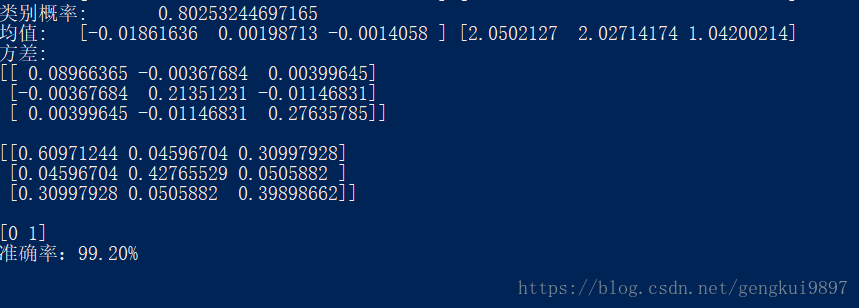
（1）手动实现

（2）sklearn库实现

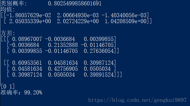
由上述两个结果可以看到，自己实现的GMM和提供的sklearn提供的GMM结果并不相同。但这并不能说明我们的实现是错误的。之所以出现上述结果，是因为EM算法会收敛到局部最优值，而不同的初值条件会收敛于不同的参数估计结果。