Wide & Deep Learning for Recommender Systems【论文记录】

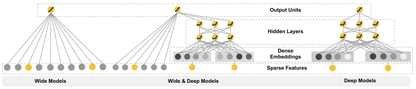
特点在于联合学习，将线性模型和神经网络联合在一起共同学习
线性模型作用于所给的特征，直接记忆专家给的有效特征
神经网络作用于所有特征，挖掘新特征，进行泛化
也就是结合 人为发现的规则和机器探索的联系

1 摘要

• Memorization of feature interactions through a wide set of cross-product feature transformations are effective and interpretable
  通过广泛的交叉乘积特征转换来记忆特征交互是有效且可解释的

• deep neural networks with embeddings can over-generalize and recommend less relevant items when the user-item interactions are sparse and high-rank.
  当用户-项目交互稀疏且秩很大时，带有 embedding 的深度神经网络可能会过度泛化并建议相关性较低的项目。

  特征非常稀疏的话，生成的 embedding 效果可能不好。如用户的偏好明显，或者商品很小众，大部分的 query-item 没有行为交互，而可能 embedding 算出的权值大于 0，导致过拟合，使得推荐效果不好

2 介绍

• A recommender system can be viewed as a search ranking system. One challenge in recommender systems, similar to the general search ranking problem, is to achieve both memorization and generalization
  推荐系统可以视为搜索排名系统，与一般搜索排名问题类似，推荐系统中的一项挑战是同时实现记忆化和泛化

• Memorization can be loosely defined as learning the frequent co-occurrence of items or features and exploiting the correlation available in the historical data
  记忆化可以大致地定义为学习项目或特征的频繁共现并利用历史数据中可用的相关性

• Generalization, on the other hand, is based on transitivity of correlation and explores new feature combinations that have never or rarely occurred in the past
  另一方面，泛化基于相关的可传递性，并探索过去从未或很少发生的新特征组合

• Embedding-based models is difficult to learn effective low-dimensional representations for queries and items when the underlying query-item matrix is sparse and high-rank, such as users with specific preferences or niche items with a narrow appeal
  当底层需求物品矩阵稀疏且秩很大时，例如具有特定偏好的用户或吸引力较小的小众项目，基于嵌入的模型很难学习有效的需求和物品的低维表示形式

• linear models with cross-product feature transformations can memorize these “exception rules” with much fewer parameters.
  具有交叉乘积特征转换的线性模型可以用更少的参数来记住这些“例外规则”。

  这句话表示了浅模型可以用来记住一些“特殊规则”，且参数更少

3 推荐系统概述

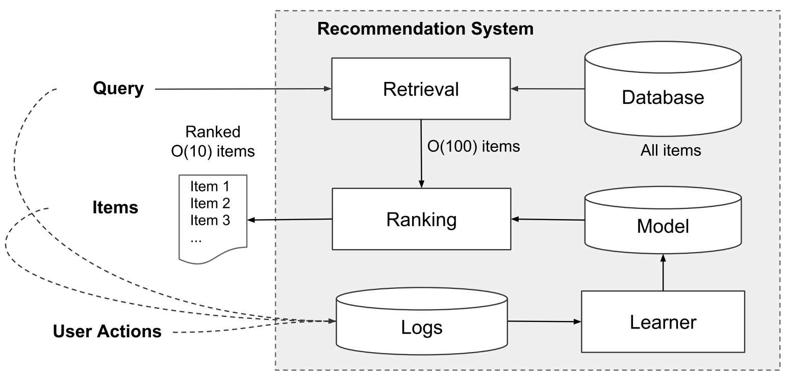
• These user actions, along with the queries and impressions, are recorded in the logs as the training data for the learner.
  这些用户操作连同查询和印象将将作为学习的训练数据记录在日志中

• the first step upon receiving a query is retrieval. The retrieval system returns a short list of items that best match the query using various signals, usually a combination of machine-learned models and human-defined rules.
  接收到查询请求的第一步是检索（召回）。 检索系统使用各种信号（通常是机器学习的模型和人工定义的规则的组合）返回简短匹配的项目清单。

• After reducing the candidate pool, the ranking system ranks all items by their scores. The scores are usually $P(y|x)$, the probability of a user action label y given the features x, including user features (e.g., country, language, demographics), contextual features (e.g., device, hour of the day, day of the week), and impression features (e.g., app age, historical statistics of an app)
  减少候选库后，排序系统将所有项目按其得分进行排名。 分数通常为 $P(y|x)$，即给定特征 x 时用户动作标签 y 的概率，包括用户特征（例如国家/地区，语言，人口统计信息），上下文特征（例如设备，一天中的某天，一天中的某天） 以及每周的展示次数功能（例如，应用程序的使用期限，应用程序的历史统计信息）

4 模型学习

4.1 宽组件

• The wide component is a generalized linear model of the form $y=w^{T}x+b$
  宽组件是 $y=w^{T}x+b$ 形式的广义线性模型

• The feature set includes raw input features and transformed features
  特征集包括原始输入特征和转换后特征

• cross-product transformation 交叉乘积转换
  ϕ k ( x ) = ∏ i = 1 d x i c k i c k i ∈ { 0 , 1 } (1) \phi_{k}(\mathbf{x})=\prod_{i=1}^{d} x_{i}^{c_{k i}} \quad c_{k i} \in\{0,1\} \tag{1} ϕk​(x)=i=1∏d​xicki​​cki​∈{ 0,1}(1) 其中 $c_{ki}$ 是一个布尔量。如 “AND(gender=female, language=en)” 是 1 当且仅当构成特征 (“gender=female” and “language=en”) 都是 1，否则就是 0

4.2 深组件

• For categorical features, the original inputs are feature strings (e.g., “language=en”). Each of these sparse, high-dimensional categorical features are first converted into a low-dimensional and dense real-valued vector, often referred to as an embedding vector.
  对于类别特征，原始输入是特征字符串（例如，“ language = en”）。首先将每一个稀疏的高维类别特征转换为低维且稠密的实值向量，通常将其称为嵌入向量。这就是 Embedding 的作用之一

• The dimensionality of the embeddings are usually on the order of O(10) to O(100).
  Embedding 向量的维数通常在 O(10) 到 O(100) 的数量级上。

• The embedding vectors are initialized randomly and then the values are trained to minimize the final loss function during model training.
  在模型训练过程中，随机初始化嵌入向量，然后训练嵌入向量，使最终损失函数最小化。

• 每个隐藏层
  $$a^{(l+1)}=f(W^{(l)}{a}^{(l)}+b^{(l)})\text{\hspace{1em}(2)}$$
  $l$ 是层数号
  $f$ 是激活函数，通常是 ReLu
  $a$，$b$，$W$ 是激活值、偏差值和模型权值

5 联合训练

• The wide component and deep component are combined using a weighted sum of their output log odds as the prediction, which is then fed to one common logistic loss function for joint training
  将宽组件和深组件的输出对数几率的加权和作为预测结果，并输入到一个共同的 logistic 损失函数进行联合训练

• there is a distinction between joint training and ensemble

  • train 方面

    • In an ensemble, individual models are trained separately without knowing each other, and their predictions are combined only at inference time but not at training time.
      在一个集成中，各个模型在不相互了解的情况下单独训练，它们的预测只在预测时组合，而在训练时不合并。

    • In contrast, joint training optimizes all parameters simultaneously by taking both the wide and deep part as well as the weights of their sum into account at training time
      相比之下，联合训练同时考虑宽，深部分以及它们的权重来同时优化所有参数

  • size 方面

    • the training is disjoint, each individual model size usually needs to be larger (e.g., with more features and transformations) to achieve reasonable accuracy for an ensemble to work
      训练是不相交的，通常每个模型的大小都需要更大（例如，具有更多的功能和变换），以实现合理的准确性以使整体工作

    • joint training the wide part only needs to complement the weaknesses of the deep part
      联合训练的宽组件只是用来弥补深组件的缺点，所以只需要比较少的 cross-product，而不是 full-size wide model

• Joint training of a Wide & Deep Model is done by back-propagating the gradients from the output to both the wide and deep part of the model simultaneously using mini-batch stochastic optimization
  宽、深组件的联合训练是利用小批量随机优化方法同时将输出梯度反向传播到模型的宽、深两部分

• In the experiments, we used Follow-the-regularized-leader (FTRL) algorithm with L1 regularization as the optimizer for the wide part of the model, and AdaGrad for the deep part
  在实验中，我们使用带有 L1 正则化的 Follow-the-regularized-leader（FTRL）算法作为模型宽组件的优化器，而 AdaGrad 作为模型深组件的优化器

• 模型的预测
  $$P(Y=1\mid \mathbf{x})=\sigma \left({\mathbf{w}}_{wide}^T[\mathbf{x},\varphi (\mathbf{x})]+{\mathbf{w}}_{deep}^T{a}^{\left(l_f\right)}+b\right)\text{\hspace{1em}(3)}$$
  $Y$ 是二分类标签
  $\sigma ()$ 是 sigmoid 函数
  $\varphi (x)$ 是原始特征 x 的交叉乘积变换
  $w_{wide}$ 是 wide 模型的权值向量
  $w_{deep}$ 是 deep 模型最后一层的激活值的权值向量

6 实现

6.1 数据生成

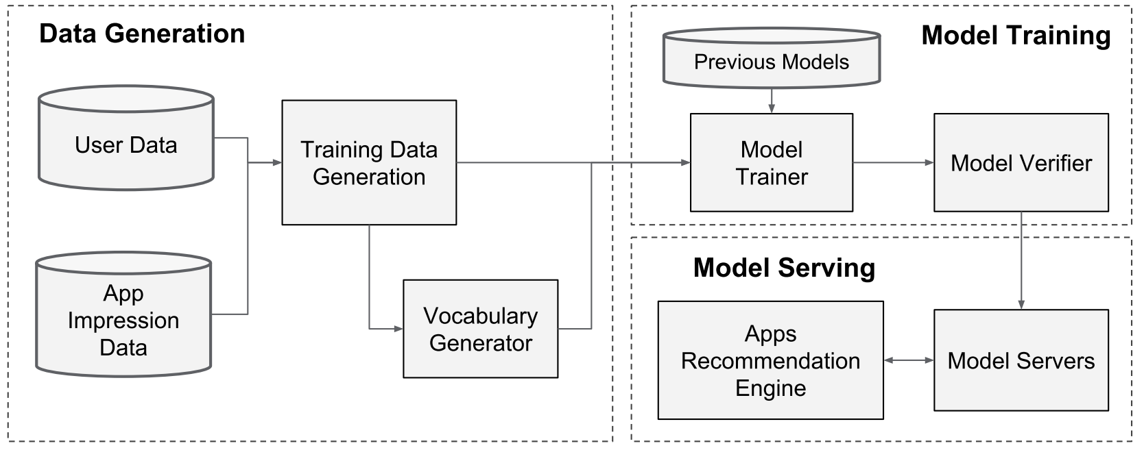
• Vocabularies, which are tables mapping categorical feature strings to integer IDs, are also generated in this stage.
  这个阶段会生成将类别特征映射到整数 ID 的词汇表

• Continuous real-valued features are normalized to [0, 1] by mapping a feature value x to its cumulative distribution function
  将实数特征归一化，并按原数字大小顺序位置（分位点）排列

6.2 模型训练

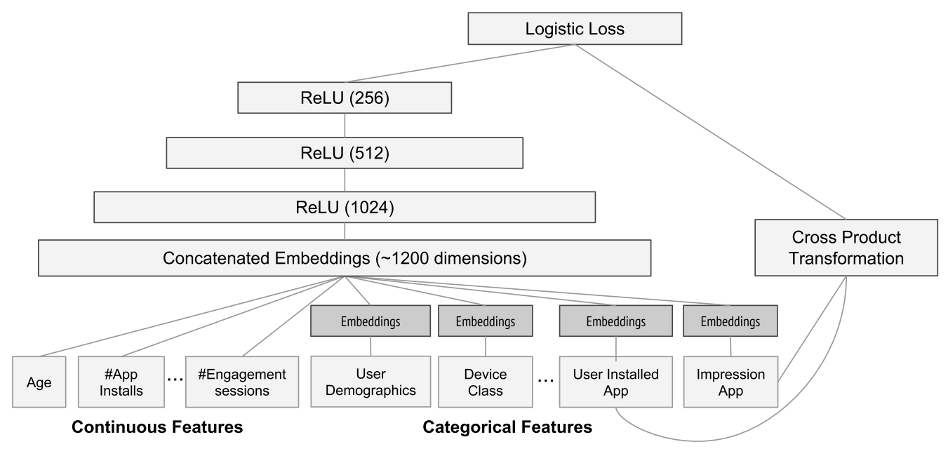
• The wide component consists of the cross-product transformation of user installed apps and impression apps
  宽组件包括用户安装的应用程序和印象产品的交叉乘积转换（选出来的特征）

• For the deep part of the model, A 32 dimensional embedding vector is learned for each categorical feature
  对于模型的较深部分，为每个分类特征学习一个32维嵌入向量

• Every time a new set of training data arrives, the model needs to be re-trained. However, retraining from scratch every time is computationally expensive and delays the time from data arrival to serving an updated model.
  每次收到一组新的训练数据时，都需要对模型进行重新训练。 但是，每次从头开始的重新训练在计算上都是昂贵的，并且会延迟从数据到达到提供更新模型的时间。

  To tackle this challenge, we implemented a warm-starting system which initializes a new model with the embeddings and the linear model weights from the previous model
  为了应对这一挑战，我们实施了热启动系统，该系统使用先前模型中的嵌入向量和线性模型权重来初始化新模型

• In order to serve each request on the order of 10 ms, we optimized the performance using multi-threading parallelism by running smaller batches in parallel, instead of scoring all candidate apps in a single batch inference step.
  为了满足10毫秒量级的每个请求，我们通过多线程并行运行来优化性能，方法是并行运行较小的批处理，而不是在单个批处理步骤中对所有候选应用程序评分。

7 总结

• Wide linear models can effectively memorize sparse feature interactions using cross-product feature transformations, while deep neural networks can generalize to previously unseen feature interactions through low dimensional embeddings
  线性模型可以使用交叉乘积特征变换有效地存储稀疏特征交互，而深度神经网络可以通过低维嵌入将其泛化到到以前看不到的特征交互

• Online experiment results showed that the Wide & Deep model led to significant improvement on app acquisitions over wide-only and deep-only models
  在线实验结果表明，与“仅宽”和“仅深”模型相比，“宽和深”模型可以显著改善应用程序的购置