logistic regression(2)

逻辑回归不仅可以做二分类，也可以来做多分类，多分类原理是基于对每个类别区别于其他类别的多个二分类来进行划分的，本质上就是多个二分类。
这里我之前存在一个思维误区，想当然认为既然是二分类，就是对两个不同的类别来进行区分，后面发现这样做多分类时按照上述的思路是存在一定问题的，因为此时构建的n个分类器之后，预测未知数据会产生n种预测结果，而如果认为二分类是就是在区别两类时，就无法确定每一次构建的二分类到底那个类别是大于阈值，那类是小于阈值了，那么多分类的设想就无法实现。
后在才恍然大悟，逻辑回归的二分类其实只是在找出正例的类别，从概率角度来解释就是认为某件事情会发生，那么这件事情发生的概论必然超过某个阈值，那么超过了我们就认为它是，否则就不是。事实上，我们只关心它是否是，它不是我们并不关心，因为确定是了之后其余的可判定为不是了。
解释有点绕口，图解会明朗一些，还是以经典的iris数据集为例子：
这里写图片描述

这里写图片描述

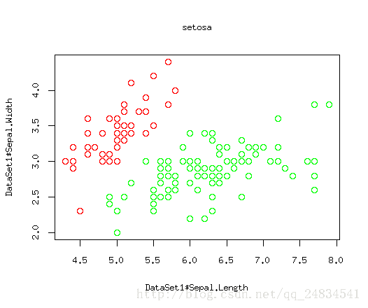
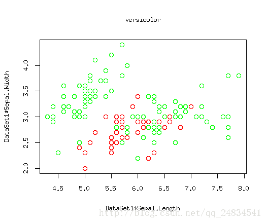
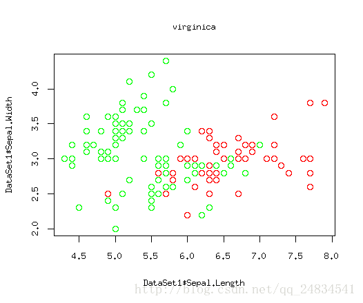
上面三幅图，红色点就是我们要关心的正例，绿色就是被剩下的部分，这里因为二维数据可以构建在散点图上比较清晰的展现出数据规律，所以我这里只选取了两个特征。如图所示，setosa类别能找到一个根直线将它于其他类别划分出来，因为versicolor 和virginica存在一定交合，从而很难被线性分割出来。当然我要阐述的问题的重点是这三幅图相当于三个分类器，而我们关心的则是每个分类是否能将红色的点区分出来。

再来看那个经典的sigmoid函数:
这里写图片描述
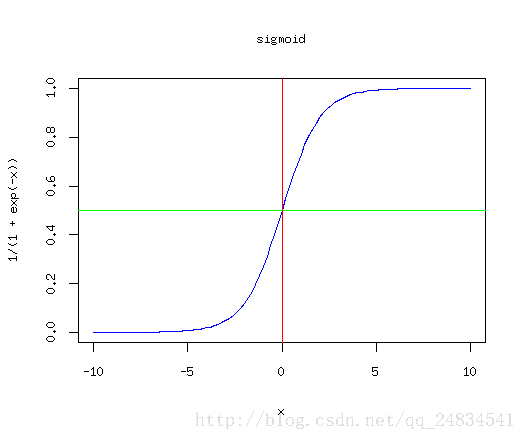
这是逻辑回归线性的映射，一个递增的函数，因此在原点越右边x轴的值对应的y值就越接近于1，换句话说就是样本被划分为正例的概率也就越大，那么对于多分类问题，就是构建出能划分出每个类别的分类器，当预测未知数据时，会进入每一个分类器，那么得到结果最大的那个作为最终的分类结果，既属于某个类别的概率最大，就认定它属于该类别。
假设离散型随机变量Y的取值集合{1, 2, 3, …., K}, 那么多分类的逻辑回归模型就是:

$P (Y = k | x) = e x p ( w k * x ) 1 + \sum K - 1 k = 1 e x p ( w k * x ), k = 1, 2, . . ., K - 1$ $\begin{align} P(Y = k | x) = \frac{exp(w_k*x)} {1 + \sum_{k=1}^{K-1}exp(w_k * x)}, k = 1,2,...,K-1 \end{align}$
$P (Y = K | x) = 1 1 + \sum K - 1 k = 1 e x p ( w k * x ), k = 1, 2, . . ., K - 1$ $\begin{align} P(Y = K | x) = \frac{1} {1 + \sum_{k=1}^{K-1}exp(w_k * x)}, k = 1,2,...,K-1 \end{align}$

得到概率最大的分类器：

h m a x (x) = arg max h (i) θ (x)

$\begin{align} h_{max}(x) = \arg\max h_\theta^{(i)}( x) \end{align}$

理论和原理阐述到此为止，下面上代码。还是基于Rcpp下的C++代码，但是对之前的二分类做了改进，将二分类拓展至多分类，同时在R中来进行调用预测。

#include <Rcpp.h>
#include <math.h>
#include <set>

using namespace Rcpp;
using namespace std;

// [[Rcpp::export]]
double sigmoid(double z)
{
  return exp(z) / (1+exp(z));
}

//[[Rcpp::export]]
double cost_func(NumericMatrix x, NumericVector y, NumericVector weight, 
                 const int nrow, const int ncol){
   double loss = 0;
   double  final_loss = 0;
   for (int i = 0;i < nrow;++i){
     double h = 0;
     for (int j = 0;j < ncol;j++){
       h += weight[j] * x(i, j);
     }
     loss += (y[i] * log(sigmoid(h)) + (1 - y[i]) * log(1 - sigmoid(h)));
   }
   final_loss = - ((double) 1 / nrow) * loss;
   cout << "error: "<< final_loss << endl;
   return final_loss;
}

// [[Rcpp::export]]
NumericVector gradient_descent(NumericMatrix x, NumericVector y, NumericVector weight, 
                               const int nrow, const int ncol, double learning_rate, double lambda){
  NumericVector sum(ncol);
  // calculate sum
  for (int k = 0;k < ncol; ++k){
    for (int i = 0;i < nrow; ++i){
      double h = 0;
      for (int j = 0;j < ncol;j++){
        h += weight[j] * x(i, j);
      }
      sum[k] += (y[i] - sigmoid(h)) * x(i, k);
    }
  }
  // update weight
  for (int k = 0; k < ncol; ++k){
    weight[k] += learning_rate * ((double) 1 / nrow) * sum[k];
  }
  return weight;
}

// [[Rcpp::export]]
NumericVector Logitis(NumericMatrix x, const int nrow, const int ncol, 
                      NumericVector y, double learning_rate, int max_iter, 
                      double min_error, double lambda){
  // i nrow  
  // j ncol 
  // x = i X j  
  set<double> s_y; 

  // cheak label count
  for (int i = 0; i < nrow; ++i) {
    s_y.insert(y[i]);
  }
  set<double>::iterator it = s_y.begin();
  set<double>::iterator it_end = s_y.end(); 
  if (s_y.size() < 2){
    cout << "Must be two class for model..." << endl;
  }
  else if (s_y.size() == 2) {
    int iter = 0;
    double loss = 10;
    // inital weight
    NumericVector weight(ncol); 
    for (int j = 0; j < ncol; ++j) {
      weight[j] = 1.0; 
    }
    // set iter times and control error
    while (iter < max_iter && loss > min_error){
      // Batch gradient descent
      weight = gradient_descent(x, y, weight, nrow, ncol, learning_rate, lambda);
      // Square error
      loss = cost_func(x, y, weight, nrow, ncol);
      iter++;
    }
    return weight;

  } else if (s_y.size() > 2 && s_y.size() <= 100){
    int k = 0;
    int labels = s_y.size();
    int weight_len = labels * ncol;
    NumericMatrix weight_matrix(labels, ncol);
    NumericVector weight_vector(weight_len);
    for (; it != s_y.end(); ++it){
      int iter = 0;
      double loss = 10;
      // inital weight
      NumericVector weight(ncol); 
      for (int j = 0; j < ncol; ++j){
        weight[j] = 1.0; 
      }
      NumericVector t_y(nrow);
      for (int i = 0; i < nrow; ++i){
        t_y[i] = 0; 
      }
      // labels 0-1
      for (int i = 0; i < nrow; ++i){
        if (y[i] == *it){
          t_y[i] = 1;
        } else {
          t_y[i] = 0;
        }
      }
      // set iter times and control error
      while (iter < max_iter && loss > min_error){
        // Batch gradient descent
        weight = gradient_descent(x, t_y, weight, nrow, ncol, learning_rate, lambda);
        // Square error
        loss = cost_func(x, t_y, weight, nrow, ncol);
        iter++;
      }
      cout << endl;
      // save weight in matrix
      for (int j = 0;j < ncol; ++j){
        weight_matrix(k, j) = weight[j];
      }
      k++;
    }
    int n = 0;
    // read in vector
    for (int i = 0;i < labels;i++){
      for (int j = 0;j< ncol;j++){
        if (n < labels * ncol){
          weight_vector[n] = weight_matrix(i, j);
          n++;
        } 
      }
    }
    return weight_vector;
  } else {
    cout << "too much Classifier type for this model..." << endl;
  }
}
// [[Rcpp::export]]
NumericVector Logitis_predict(NumericMatrix x, NumericVector weight, 
                              const int nrow, const int ncol){
  if (weight.size() == ncol){
    // predict labels equals two
    NumericVector Y(nrow);
    for (int i = 0; i < nrow; i++){
      double h = 0;
      for (int j = 0; j < ncol; j++){
        h += weight[j] * x(i, j);
      }
      if (sigmoid(h) >= 0.5) {
        Y[i] = 1;
      } else {
        Y[i] = 0;
      }
    }
    return Y;

  } else {
    // predict labels equals more than two
    int n = 0;
    int labels_nrow = (double) weight.size() / ncol;
    NumericVector Y(nrow);
    NumericMatrix weight_matrix(labels_nrow, ncol);
    for (int i = 0; i < labels_nrow; ++i){
      for (int j = 0; j < ncol; ++j){
          weight_matrix(i, j) = weight[n];
          n++;
      }
    }
      for (int i = 0; i < nrow; i++){
        NumericVector h(labels_nrow);
        for (int k = 0; k < labels_nrow; ++k){
          for (int j = 0; j < ncol; j++){
            h[k] += weight_matrix(k, j) * x(i, j);
        }
        Y[i] = which_max(h) + 1;   
      }
    }
    return Y;
  }
}

代码将，sigmoid函数，梯度下降，损失函数误差部分分别抽离原Logitis函数，在实现代码时才真正对算法有更进一步的了解，实际上逻辑回归只接受0-1值作为预测变量，之前用现成的库并没有在意这些细节问题，因为R中预测变量会作为因子变量来对待。

下面还是以R来测试模型效果, 以后会尝试用 python 来调用测试模型效果。

library(Rcpp)
# my logitis
sourceCpp(file = "logitis.cpp")
## way 1 #####################################################################
DataSet1 <- iris
DataSet1$Species <- ifelse(DataSet1$Species == "setosa", 1, 0)
index1 <-  sample(2, nrow(DataSet1), replace = TRUE, prob = c(0.7, 0.3))
# train1 data 
trainData1 <- DataSet1[index1 == 1, ]
train1_X <- as.matrix(trainData1[, -5])
train1_Y <- trainData1[, 5]
# test1 data
testData1 <- DataSet1[index1 == 2, ]
test1_X <- as.matrix(testData1[, -5])
test1_Y <- testData1[, 5]
#### _________________________________________________________________________________________ 
# weight
weight1 <- Logitis(train1_X, nrow(train1_X), ncol(train1_X), train1_Y, 0.1, 100, 0.01, 0.01)
# predict 
pred_y1 <- Logitis_predict(test1_X, weight1, nrow(test1_X), ncol(test1_X))
# Evaluation
evaluation_result <- pred_y1 == test1_Y
cat("Accuracy: ", length(evaluation_result[evaluation_result == TRUE]) / length(test1_Y), "\n")
## way 2 #####################################################################
DataSet2 <- iris
DataSet2$Species <- ifelse(DataSet2$Species == "versicolor", 1, 0)
index2 <-  sample(2, nrow(DataSet2), replace = TRUE, prob = c(0.7, 0.3))
# train2 data
trainData2 <- DataSet2[index2 == 1, ]
train2_X <- as.matrix(trainData2[, -5])
train2_Y <- trainData2[, 5]
# test2 data
testData2 <- DataSet2[index2 == 2, ]
test2_X <- as.matrix(testData2[, -5])
test2_Y <- testData2[, 5]
#### _________________________________________________________________________________________ 
# weight
weight2 <- Logitis(train2_X, nrow(train2_X), ncol(train2_X), train2_Y, 0.1, 100, 0.01, 0.01)
# predict 
pred_y2 <- Logitis_predict(test2_X, weight2, nrow(test2_X), ncol(test2_X))
# Evaluation
evaluation_result <- pred_y2 == test2_Y
cat("Accuracy: ", length(evaluation_result[evaluation_result == TRUE]) / length(test2_Y), "\n")
# way 3 ###############################################################################
DataSet3 <- iris
DataSet3$Species <- ifelse(DataSet3$Species == "virginica", 1, 0)
index3 <-  sample(2, nrow(DataSet3), replace = TRUE, prob = c(0.7, 0.3))
# train2 data
trainData3 <- DataSet3[index3 == 1, ]
train3_X <- as.matrix(trainData3[, -5])
train3_Y <- trainData3[, 5]
# test2 data
testData3 <- DataSet3[index3 == 2, ]
test3_X <- as.matrix(testData3[, -5])
test3_Y <- testData3[, 5]
#### _________________________________________________________________________________________ 
# weight
weight3 <- Logitis(train3_X, nrow(train3_X), ncol(train3_X), train3_Y, 0.1, 100, 0.01, 0.01)
# predict 
pred_y3 <- Logitis_predict(test3_X, weight3, nrow(test3_X), ncol(test3_X))
# Evaluation
evaluation_result <- pred_y3 == test3_Y
cat("Accuracy: ", length(evaluation_result[evaluation_result == TRUE]) / length(test3_Y), "\n")
# way 4 ################################################################################
DataSet4 <- iris
levels(DataSet4$Species) <- c(1L, 2L, 3L)
DataSet4$Species <- as.integer(DataSet4$Species)
index4 <-  sample(2, nrow(DataSet4), replace = TRUE, prob = c(0.7, 0.3))
# train3 data 
trainData4 <- DataSet4[index4 == 1, ]
train4_X <- as.matrix(trainData4[, -5])
train4_Y <- trainData4[, 5]
# test3 data
testData4 <- DataSet4[index4 == 2, ]
test4_X <- as.matrix(testData4[, -5])
test4_Y <- testData4[, 5]
#### _________________________________________________________________________________________ 
# weight
weight4 <- Logitis(train4_X, nrow(train4_X), ncol(train4_X), train4_Y, 0.1, 100, 0.01, 0.01)
# predict 
pred_y4 <- Logitis_predict(test4_X, weight4, nrow(test4_X), ncol(test4_X))
# Evaluation
evaluation_result <- pred_y4 == test4_Y
cat("Accuracy: ", length(evaluation_result[evaluation_result == TRUE]) / length(test4_Y), "\n")

代码还是以iris数据集为例，原数据集的分类变量是有三类，但是为了做对比测试，way1～way3 将每个类别构建出能分类出响应类别的二分类的分类器，way4 构建出多分类分类器来进行分类。

weight1
# [1]  0.2275081  2.1597683 -2.7285473 -0.6074706
weight2
# [1]  0.7003674 -1.6003702  0.3715433 -1.1510675
weight3
# [1] -2.442947 -1.727265  3.071421  3.192652
weight4
# [1]  0.21527578  2.14921377 -2.70570262 -0.61643457  1.08689368 -2.04457661  0.00909365 -0.87211218 -2.50815637 -1.71569424  3.24941125  3.03972232  2.7292319  2.7982725

weight1， weight2， weight3分别代表各自分类器训练出来的模型权重，weight4 是多分类模型训练出来的模型权重，可以明显看出 weight4 事实上就是 weight1， weight2， weight3的集合。只是因为是分别训练的，因此在数值上有一定差异。

# way 1
# Accuracy:  1
# way 2
# Accuracy:  0.5 
# way 3
# Accuracy:  0.974359 
# way 4
# Accuracy:  0.9761905

前三个模型，第二个模型也就是在三个类别中识别出versicolor类别的效果很差，其余表现较为正常，之前认为是自己模型写的问题，这里使用R原生态的 glm 训练看是否存在差异。

glm <- glm(Species~., data = DataSet2, family = binomial(link = "logit"))
pred <- predict(glm, newdata = as.data.frame(test2_X))
pred <- 1 / (1+exp(-pred))
pred <- ifelse(pred >= 0.5, 1, 0)
table(pred, test2_Y)
# test2_Y
# pred  0  1
#    0 25  9
#    1  6  8
(25 + 8) / (25 + 9 + 6 + 8)
# [1] 0.6875

发现原生态的模型表现会好一些，但是这里是没有专门划分出训练集，而是用所有数据来进行训练，所有抽出部分的测试数据在模型训练时候就被学习过一次，因此在对测试集进行预测时效果会有所提升，但是并没有达到预期，所以我实现的模型好似并无问题。

最后多分类的预测也到达了97%的准确率，看来效果还是符合预期。为了更科学的得出结论，尝试改变迭代次数来观测找出模型最佳迭代次数。

accuracy <- c()
iter_times <- seq(10, 1000, 10)
for (i in iter_times){
  # weight
  weight4 <- Logitis(train4_X, nrow(train4_X), ncol(train4_X), train4_Y, 0.1, i, 0.01, 0.01)
  # predict 
  pred_y4 <- Logitis_predict(test4_X, weight4, nrow(test4_X), ncol(test4_X))
  # Evaluation
  evaluation_result <- pred_y4 == test4_Y
  accuracy <- append(accuracy,length(evaluation_result[evaluation_result == TRUE]) / length(test4_Y))
  #cat("Accuracy: ", accuracy, "\n")
}
plot(iter_times, accuracy, type = "l", col="green")
title(main = "accuracy with iter_times", xlab = "iter_times", ylab = "accuracy")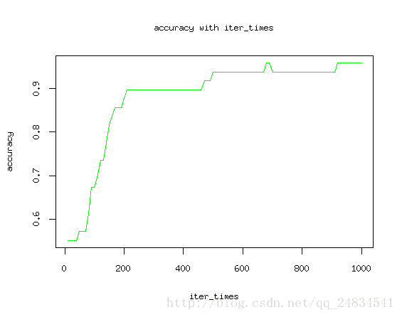

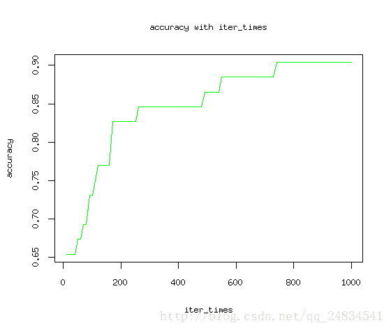
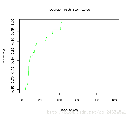
这里写图片描述

如图所示，随着迭代次数增加，模型预测结果最终收敛。
结论：通过实现逻辑回归的多分类算法，对模型有更深层级的理解，以后会尝试用其他数据集来衡量实现的算法模型的是否可靠。

<注：>这里感谢中科院生化高才学友指出我在写梯度下降时一个低级错误，不然会误导亲爱的观众。这里贴出人家公众号，有兴趣可关注。

这里写图片描述

猜你喜欢